 Click for Powerpoint Articulate Training Module Download Training Slides |
Supplemental Table of Contents |
- ProbSevere v1 training (2016): Articulate | Powerpoint
Publications and Presentations
- NOAA ProbSevere v2.0--ProbHail, ProbWind, and ProbTor, Weather and Forecasting (2020)
- The NOAA/CIMSS ProbSevere Model: Incorporation of Total Lightning and Validation, Weather and Forecasting (2018)
- An Empirical Model for Assessing the Severe Weather Potential of Developing Convection, Weather and Forecasting (2014)
- Evolution of Severe and Nonsevere Convection Inferred from GOES-Derived Cloud Properties, Journal of Applied Meteorology and Climatology (2013)
- A Satellite-Based Convective Cloud Object Tracking and Multipurpose Data Fusion Tool with Application to Developing Convection, J. Tech. (2012)
- Advances in Extracting Cloud Composition Information from Spaceborn Infrared Radiances--A Robust Alternative to Brightness Temperatures. Part I: Theory, JAMC (2010)
- ATBD for GOES-R cloud type and cloud phase algorithms (2010)
- Preliminary Evaluation of a Fused Algorithm for the Prediction of Severe Storms, AMS Annual Meeting (2014)
- NWS Great Lakes SOOs talk (2018)
- NWS Great Lakes SOOs talk (2016)
- NWS Southern Region talk (2016)
- NWS Western Region talk (2016)
- NWS Central Region talk (2015)
Statistical Model Details
How the model works
The NOAA/CIMSS ProbSevere model is a
Naive Bayesian classifier. The Naive Bayesian classifier predicts, using any number of datasets, the
probability of a 'yes' class event will occur based on the datasets used. In applying the classifier to whether a thunderstorm will first produce severe weather
in the next 60 minutes it is necesary to define the 'yes' class and 'no' class--in this application 'yes' class are storms that produce severe weather and 'no' class
are storms that do not produce severe weather.
The datasets used within the model RAP composite MUCAPE and EBS (effective bulk shear), satellite observational
predictors (normalized vertical cloud growth rate and cloud-top glaciation rate), and radar observational predictor (MRMS MESH) are collected for a set of training
data--a population of severe thunderstorms ('yes' class) and a population of non-severe thunderstorms ('no' class). Class-conditional probabilities are computed for
the range of values within each dataset for the yes and no classes. It is this training dataset that is used to compute real-time probabilties for all
storms.
In real-time, the data values for each predictor for a given storm are input into the ProbSevere model. The differences between class-conditional probabilties for the datasets
used by the model are mathematically combined to generate a final probability--the probability viewed in AWIPS-II and on this web site. The two examples below illustrate
how the class-conditional probabilities are used in the ProbSevere model to compute the final probability.
Equation
The full mathemtical equation for the naive Bayesian model is given by:

Where the final probability of a 'yes' event is given by the ratio of the product of yes-class conditional probabilities and yes-class prior probability to the product of the
yes-class conditional probabilities and yes-class prior probability plus the product of the no-class conditional probabilities and no-class prior probability.
Severe Thunderstorm Example
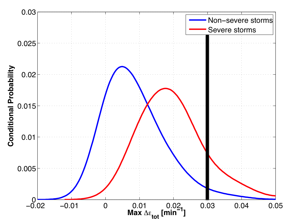
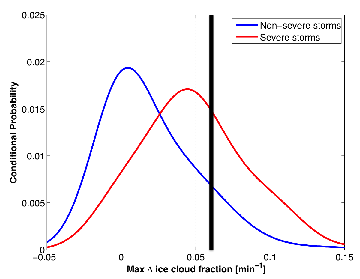
The following figures are the RAP composite MUCAPE/EBS yes-class prior probability and the class-conditional probabilitiy distributions from the
training datasets for the three observational parameters (satellite: normalized vertical growth rate and cloud-top glaciation rate) and radar: instantenous MRMS MESH).
Plotted on these figures (black) are example values for a hypothetical severe thunderstorm.
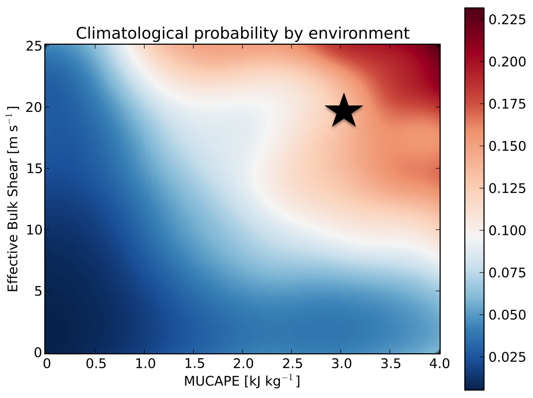
Hypothetical severe thunderstorm with 3,000 J/kg of MUCAPE and 20 m/s EBS from the RAP compsite.
Yes-class prior probability = 0.17. (No-class prior probability = 1 - 0.17 = 0.83)
Hypothetical severe thunderstorm normalized vertical growth rate of 3.0%/min. |
Hypothetical severe thunderstorm glaciation rate of 0.06/min. |
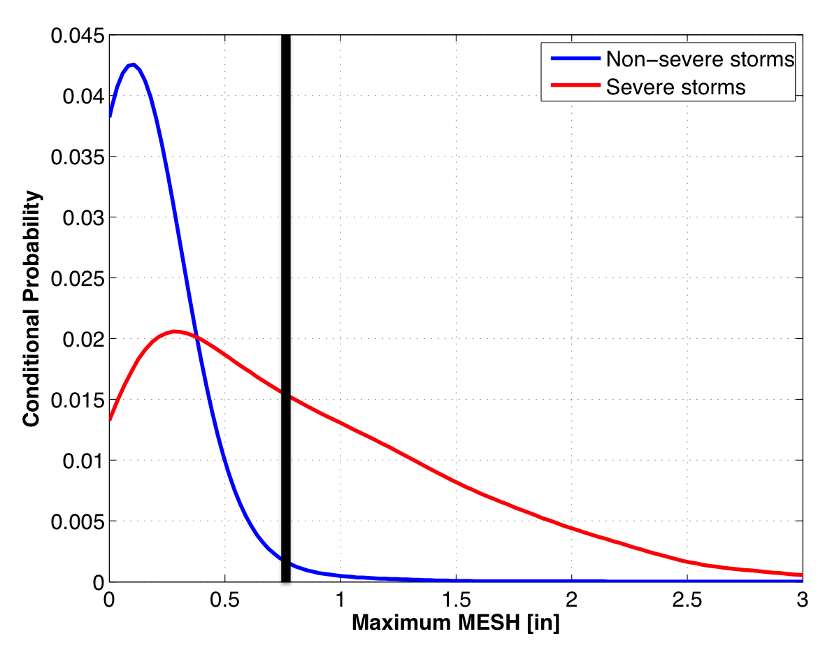
Hypothetical severe thunderstorm MRMS MESH of 0.75". |
Combining all the class-conditional probabilities and prior probabilities yields an end probability of 97%. Or this hypothetical severe thunderstorm has a
97% chance of first producing severe weather in the next 60 minutes. The very high probability is attributed to a favorable environment, strong satellite growth rates,
and a large, yet still sub-severe MRMS MESH value.

NWP Data and Temporal/Spatial Compositing
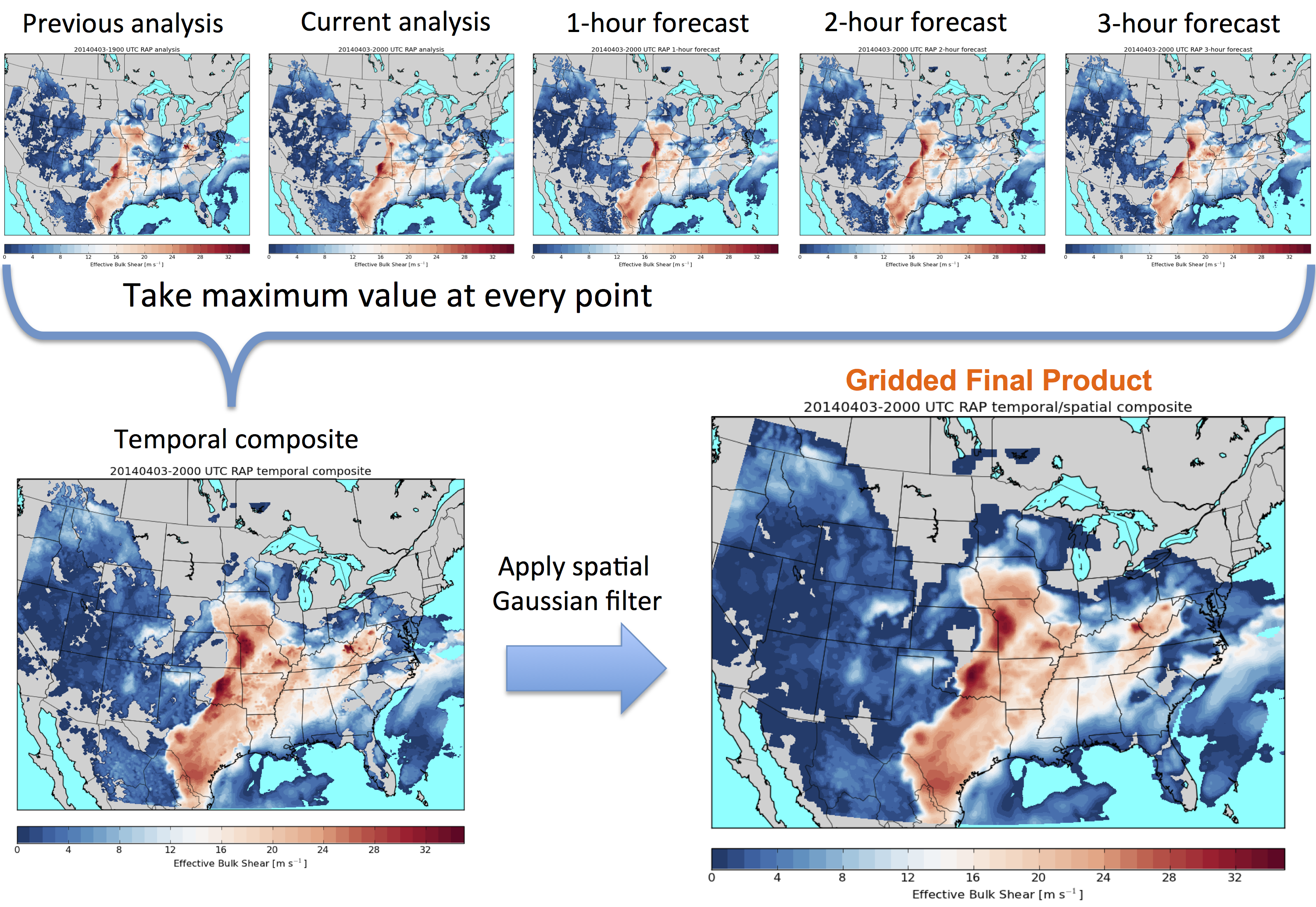
ProbSevere currently uses the Rapid Refresh model (RAP) from NCEP. The effective bulk shear (EBS) and most-unstable convective available potential energy (MUCAPE) are used as predictors in the statistical model. New RAP forecast and analysis data are available approximately every hour. Once new RAP data are available, the EBS and MUCAPE fields are computed for every gridpoint for the analysis grid, as well as the 1-, 2-, and 3-hour forecasts.
Next, for each grid point, the maximum EBS (or MUCAPE) is taken over the previous hour analysis (computed previously), the current analysis, and the 1-, 2-, and 3-hour forecasts (just computed). This "off-centered" approach is implemented since RAP data have about a one hour latency. Thus, the 1-hour forecast is approximately valid at the time the data are delivered. After the temporal compositing is complete, a spatial filter is applied, which has a Gaussian kernel. The temporal compositing and spatial smoothing of the RAP data is performed in an effort to mitigate placement and phasing errors inherent in NWP data.
Back to Table of Contents
Satellite Data and Products
The NOAA/CIMSS ProbSevere model utilizes GOES satellite imagery for both identifying and tracking cloud clusters as well as quantifying growth rates of clouds. Below
is an example of GOES cloud cluster identification and tracking for a developing thunderstorm over the Texas panhandle. The top row of images is IR-window brightness temperatures and the
bottom row are the same images with an illustration of how cloud clusters are identified and tracked by the computer.
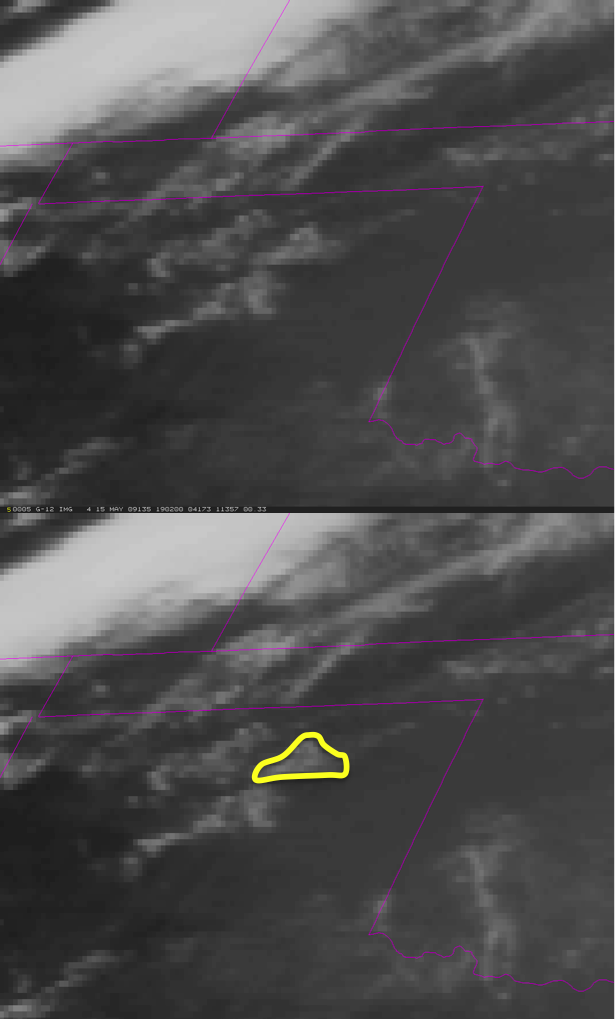
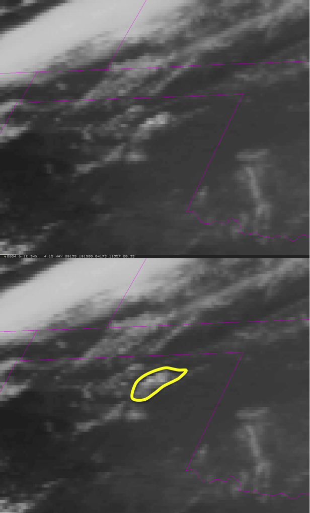
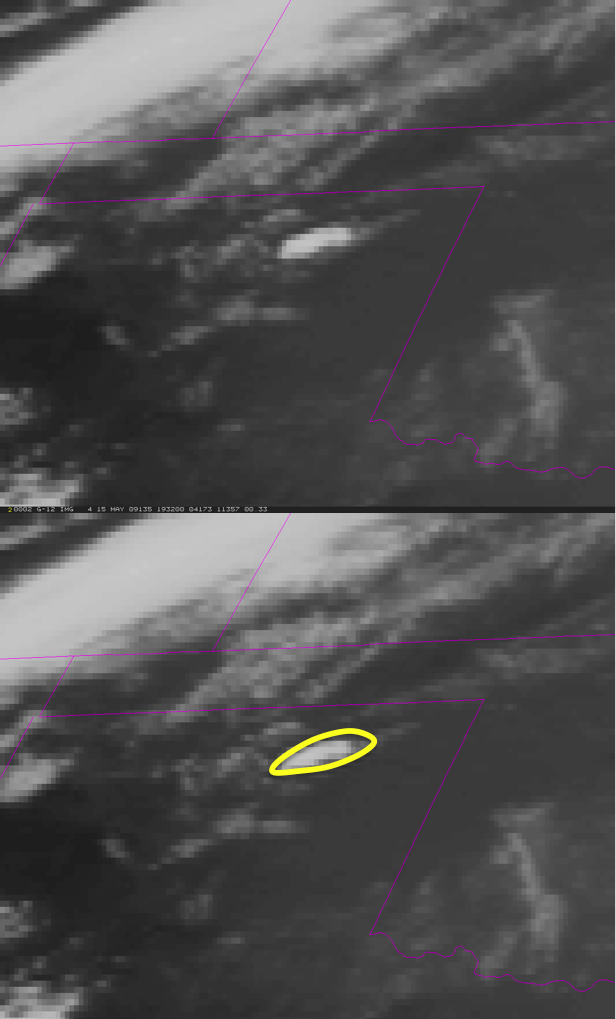
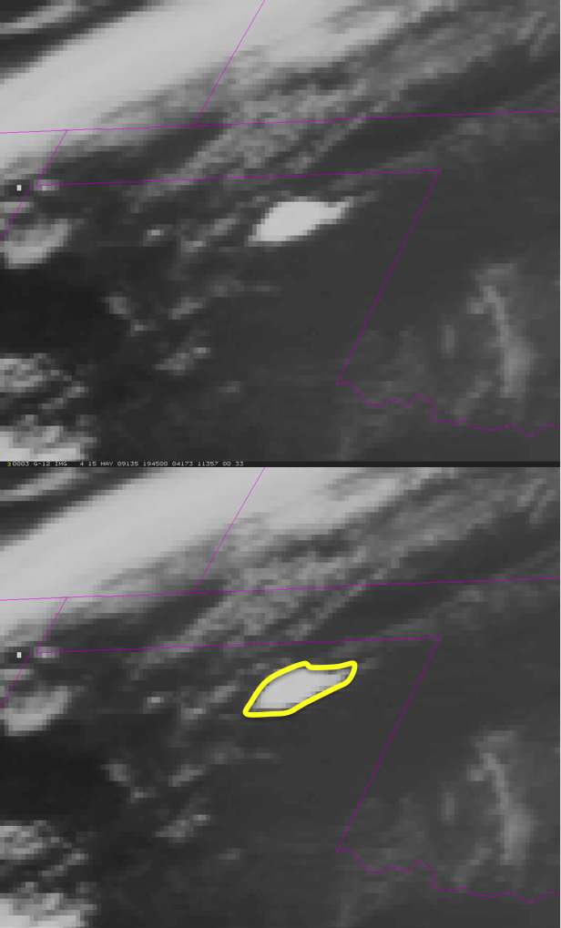
The satellite tracking uses infrared data--so the tracking is the same day and night. Within each cloud cluster the computer identifies and tracks, two satellite growth rates are computed: the normalized vertical growth rate and the cloud-top glaciation rate. The normalized vertical growth rate uses a field known as the top of troposphere emissivity (Pavolonis 2010). The vertical growth rate computed using this field is analagous to brightness temperature cooling rates, except the growth rates are normalized for varying tropospheric depth/tropopause height, while raw brightness temperature data are not. The cloud-top glaciation rate uses GOES/GOES-R cloud phase/type algorithm output to characterize how quickly the cloud-tops change from water phase to ice phase. The statistical model details shows how these two growth rates, along with radar and NWP data are used within the NOAA/CIMSS ProbSevere model.
Back to Table of Contents
Radar Data and Products
The NOAA/CIMSS ProbSevere model heavily leverages the Multi-Radar Multi-Sensor (MRMS) products developed at NOAA-NSSL and OU-CIMMS. By using multiple radars to sample weather, gaps in radar coverage due to things such as terrain blockage, the "cone of silence", and the radar beam overshooting weather at far ranges may be mitigated. Furthermore, combining multiple estimates of radar moments at any particular point can give a better final estimate. Multiple radar surveillance of weather can also provide more frequent updates. The ProbSevere model updates at the MRMS frequency, which is approximately every 2 minutes.
MRMS merged reflectivity is used to identify and track storms in radar imagery, using the Warning Decision Support System -- Integrated Information (WDSS-II). WDSS-II automatically identifies storms using an enhanced watershed algorithm and tracks storms by using methods to match identified objects in consecutive image pairs.
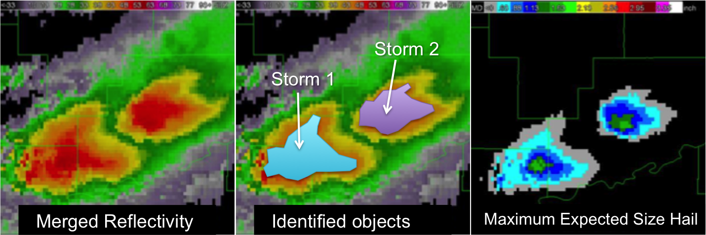
Figure is adapted from OU-CIMMS images.
Once storm objects are tracked in radar imagery, the Maximum Expected Size of Hail (MESH) is extracted from the spatial bounds of the objects. MESH is empirically derived from the Severe Hail Index (SHI), which is essentially a thermally weighted vertical integration of reflectivity above the melting level. Several recent studies have shown that MESH has some skill for identifying the presence of severe hail in storms. Please see Witt et al. (1998) for a more complete description of MESH and SHI. The instantaneous maximum MESH is used as a predictor in the ProbSevere model.
Back to Table of Contents
Model Performance
The NOAA/CIMSS ProbSevere model has been manually evaluated for about 120 days in 2014 and 2016. This evaluation encompassed over 3,200 severe storms and 61,500 non-severe storms across the CONUS. Non-severe storms were automatically identified, objectively, while severe storms were identified by manual analsyis, requiring the presence of a preliminary LSR in close proximity and time to ProbSevere objects. Please see Cintineo et al. (2018) for a complete description and analysis of the validation procedures and their results.

ProbSevere skill scores for the entire validation as a function of forecast probability threshold on a storm-by-storm basis and (right) a reliability diagram of ProbSevere skill, computed for the aggregation of every 2-min ProbSevere probability forecast. Note that the yaxis of the inset graph in (b) is log scaled.

ProbSevere, ProbSevere without the total lightning/EBShear predictor, and NWS skill scores and median lead time to initial LSR. The ProbSevere metrics are measured from the 80% forecast probability threshold.
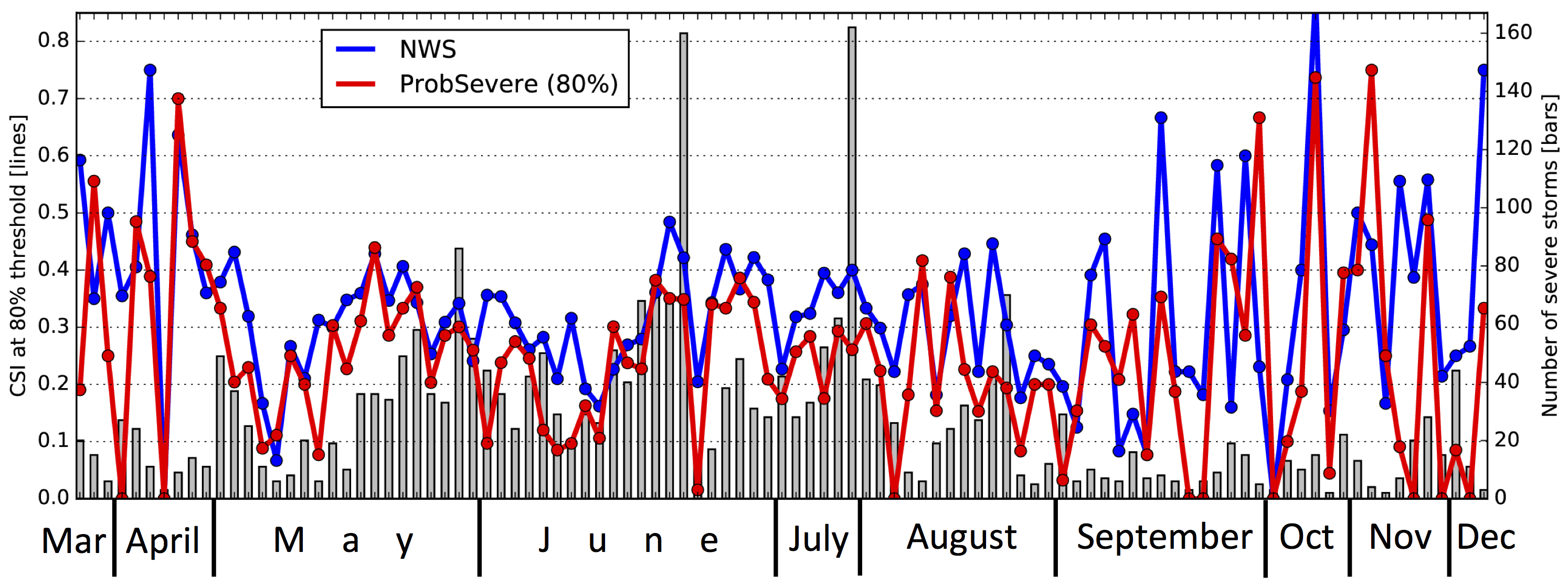
A time series of ProbSevere CSI at the 80% forecast probability threshold and NWS CSI to initial LSRs (lines) and the number of severe storms analyzed on each day (bars). The time series covers a portion of the annual cycle for 2016 only.
Please click here for spatial verification of aggregated NWS WFOs.
Back to Table of Contents