
GOES-15 0.63 µm visible channel images (Animated GIF | MP4 movie | YouTube video | QuickTime movie) showed the decoupling of the upper-level and lower-level circulations of Tropical Storm Karina... Read More
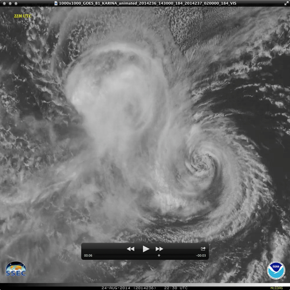
GOES-15 0.63 µm visible channel images (click to play Animated GIF)
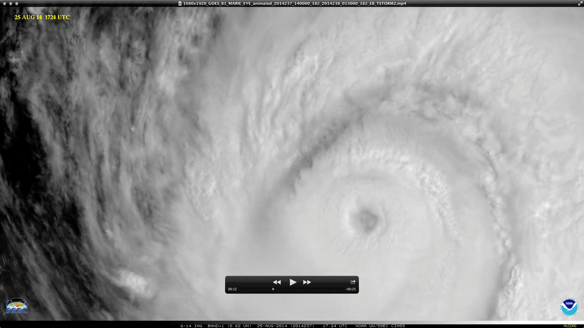
GOES-15 0.63 µm visible channel images (Animated GIF | MP4 movie | YouTube video | QuickTime movie) showed the decoupling of the upper-level and lower-level circulations of Tropical Storm Karina in the East Pacific Ocean on 24 August 2014. This decoupling was caused by strong wind shear along the western periphery of Category 5 Hurricane Marie, which was located to the east-southeast of Karina (large-scale view). Kudos to Dennis Chesters (NASA/Goddard) for bringing this interesting case to our attention (and providing the QuickTime movie linked to above).
The corresponding GOES-15 10.7 µm IR channel images (Animated GIF | MP4 movie | YouTube video) showed the cold clouds (red to black to white to purple color enhancement) associated with the upper-level circulation moving northward and quickly dissipating; the signature of the warmer clouds (darker cyan color enhancement) associated with the lower-level circulation can also be seen emerging from beneath the cold cloud shield and moving eastward.
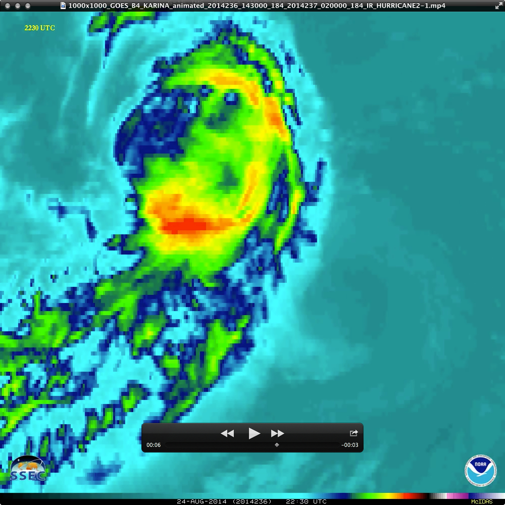
GOES-15 10.7 µm IR channel images (click to play Animated GIF)
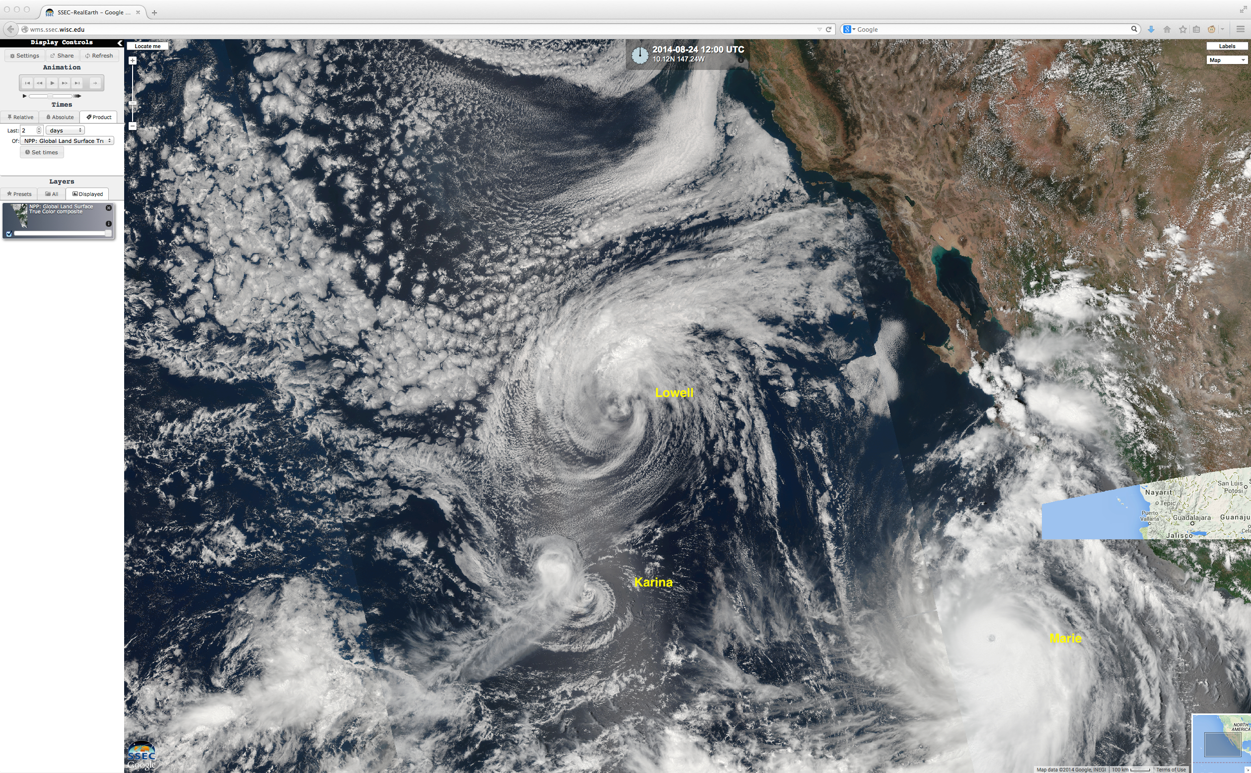
A closer view provided by a Suomi NPP VIIRS true-color Red/Green/Blue (RGB) image from the SSEC RealEarth web map server (below) showed the separation of the upper-level and lower-level circulations around 21:53 UTC.
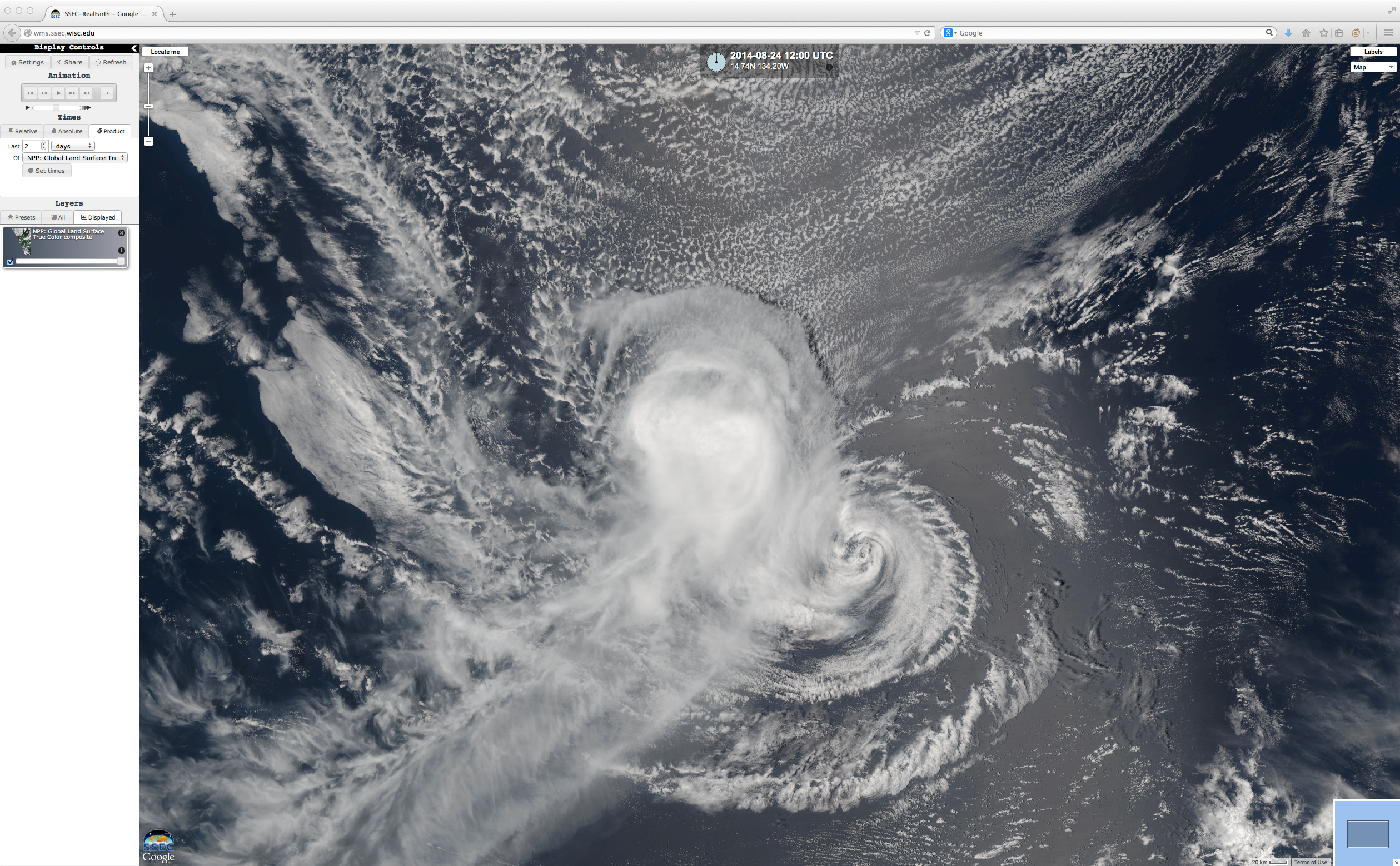
Suomi NPP VIIRS true-color RGB image
A sequence of 4 images (15, 18, 21, and 00 UTC) from the CIMSS Tropical Cyclones site (below) shows GOES-15 6.5 µm water vapor channel images with overlays of deep-layer wind shear (derived from satellite winds). To the east of Karina (which was located in the center of the images), the large anticylcone aloft associated with Category 5 Hurricane Marie can be seen, with increasing vales of southeasterly wind shear moving over Karina.
15 UTC GOES-15 6.5 µm water vapor images with overlays of deep layer wind shear
The 3 image comparisons below show the separation of the centers of upper-level divergence (yellow) and lower-level convergence (cyan) as the decoupling process was occurring at 18 UTC, 21 UTC, and 00 UTC.
18 UTC: GOES-15 6.5 µm water vapor image with upper-level divergence (yellow) and GOES-15 10.7 µm IR image with lower-level convergence (cyan)
21 UTC: GOES-15 6.5 µm water vapor image with upper-level divergence (yellow) and GOES-15 10.7 µm IR image with lower-level convergence (cyan)
00 UTC: GOES-15 6.5 µm water vapor image with upper-level divergence (yellow) and GOES-15 10.7 µm IR image with lower-level convergence (cyan)
===== 25 August Update =====
GOES-15 0.63 µm visible channel images, with Metop ASCAT surface scatterometer winds
Even though the southeastward-moving low-level circulation of Karina had been downgraded to a Tropical Depression with 30 knot winds, there was still an impressive burst of convection just west of the center as it began to move back over warmer water on 25 August. Metop ASCAT surface scatterometer winds (above) showed a small pocket of winds in the 30.0-39.9 knot range (green wind barbs) at 18:29 UTC.
There were also some Tropical Overshooting Top (TOT) targets detected within the convective burst (below); TOT symbols: Red = 0-1 hour previous, Green = 1-2 hours previous, Blue = 2-3 hours previous.
GOES-15 Infrared – Water Vapor difference product, and Tropical Overshooting Tops product (TOT symbols: Red = 0-1 hour previous, Green = 1-2 hours previous, Blue = 2-3 hours previous)
View only this post
Read Less

