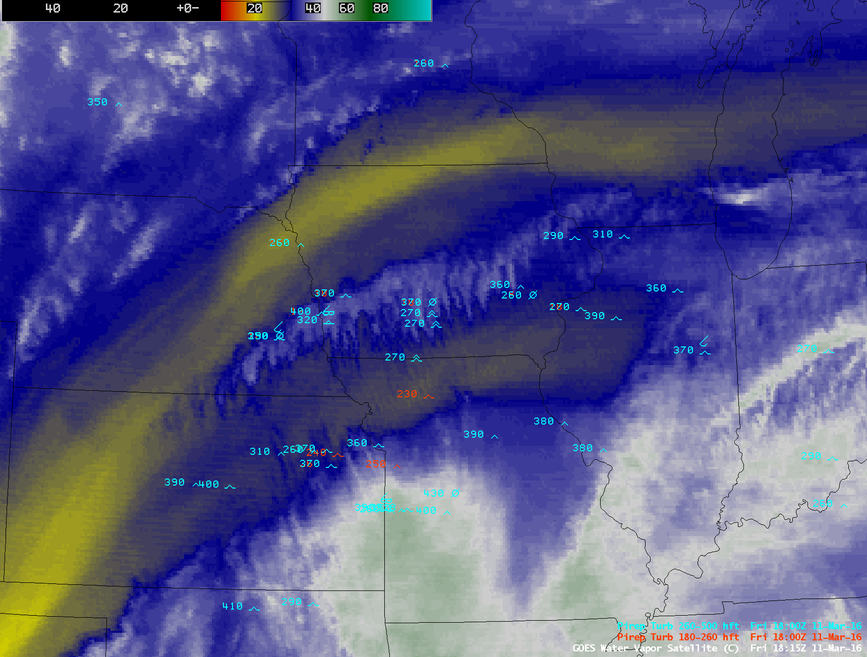
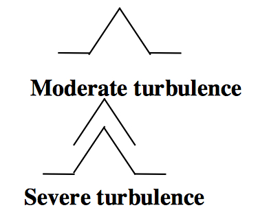
There were numerous pilot reports of Moderate to Severe turbulence (symbols) over much of the Midwest on 11 March 2016, as shown plotted on 4-km resolution GOES-13 (GOES-East) Water Vapor (6.5 µm) images (above). A packet of transverse banding cloud features developed over eastern Kansas after about 1515 UTC, and moved northeastward... Read More
![GOES-13 Water Vapor (6.7 µm) images with Pilot Reports of turbulence [click to play animation]](https://cimss.ssec.wisc.edu/satellite-blog/wp-content/uploads/sites/5/2016/03/US_Water_Vapor_20160311_1815.png)
GOES-13 Water Vapor (6.7 µm) images with Pilot Reports of turbulence [click to play animation]
There were numerous pilot reports of Moderate to Severe turbulence (
symbols) over much of the Midwest on
11 March 2016, as shown plotted on 4-km resolution GOES-13
(GOES-East) Water Vapor (6.5 µm) images
(above). A packet of transverse banding cloud features developed over eastern Kansas after about 1515 UTC, and moved northeastward over northwestern Missouri/southeastern Nebraska/Iowa/northern Illinois/southern Wisconsin during the day.
The transverse banding cloud filaments showed up with a bit more clarity on a 1-km resolution Aqua MODIS Water Vapor (6.7 µm) image at 1919 UTC (below).
![Aqua MODIS Water Vapor (6.7 µm) image [click to enlarge]](https://cimss.ssec.wisc.edu/satellite-blog/wp-content/uploads/sites/5/2016/03/MODIS_WV_20160311_1919.png)
Aqua MODIS Water Vapor (6.7 µm) image [click to enlarge]
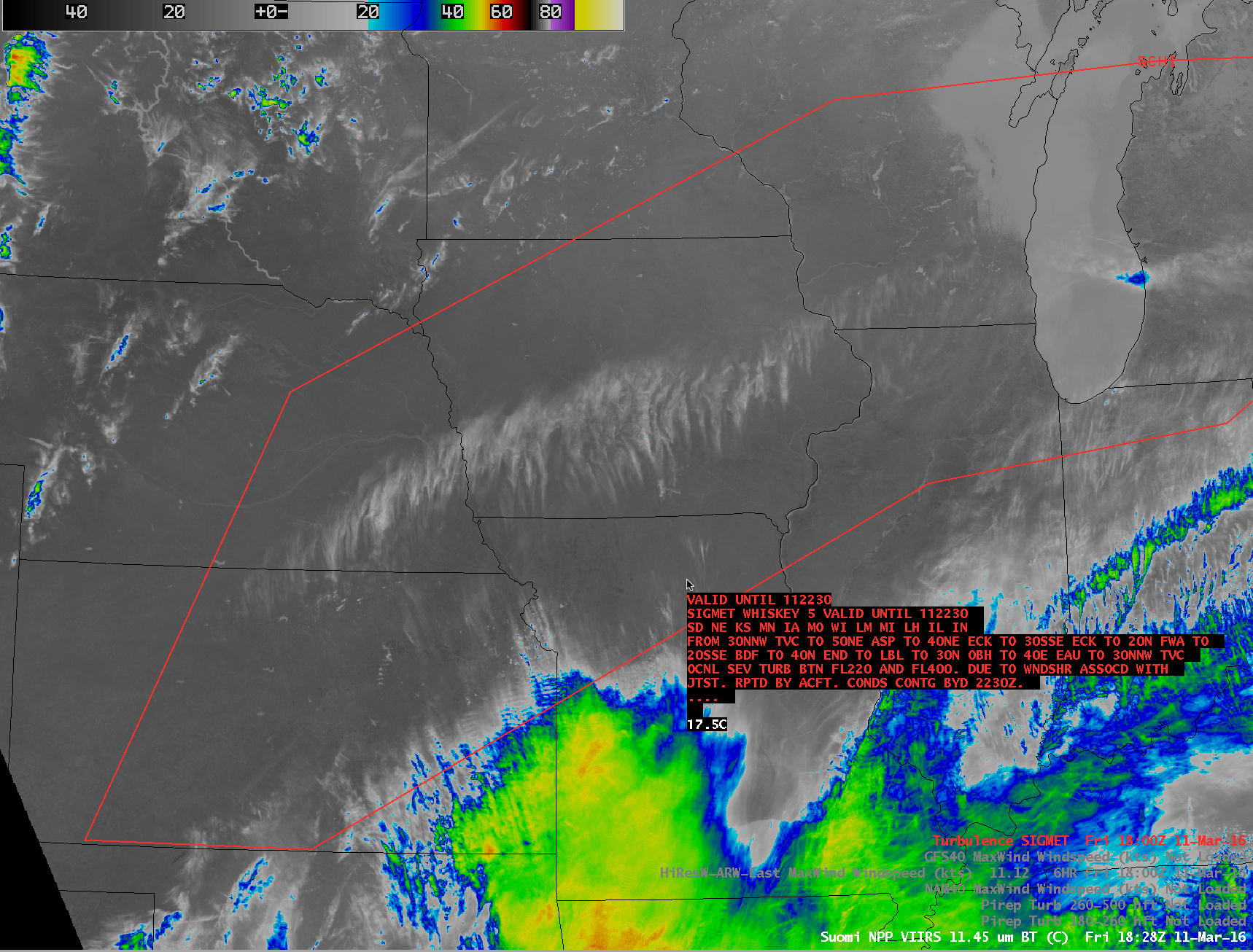
A MODIS Cirrus (1.4 µm) image at 1738 UTC
(below) was also a very effective tool for helping to visualize the transverse banding cloud filaments. A Turbulence
SIGMET had been issued at 1433 UTC for much of the region, due to wind shear associated with jet steam aloft. Many of the pilot reports were noted to be Clear Air Turbulence (CAT), with one describing the severe turbulence encounter as “
one jolt“. It can be seen from the GFS model isotachs of Maximum Wind that the reports of turbulence occurred within the entrance region of a curved jet stream segment, which are areas that favor the development of strong vertical and horizontal wind shear responsible for turbulence.
![Terra MODIS "Cirrus" (1.38 µm) image with Turbulence SIGMET, Pilot Reports of turbulence, and GFS Max Wind isotachs [click to enlarge]](https://cimss.ssec.wisc.edu/satellite-blog/wp-content/uploads/sites/5/2016/03/160311_1738utc_modis_cirrus_sigmet_pireps_gfs_maxwinds_anim.gif)
Terra MODIS “Cirrus” (1.38 µm) image with Turbulence SIGMET, Pilot Reports of turbulence, and GFS Max Wind isotachs [click to enlarge]
On a comparison of 1-km resolution Aqua MODIS Visible (0.65 µm) and Infrared Window (11.0 µm) images at 1919 UTC
(below), the very thin nature of the transverse banding cirrus cloud features made them difficult to identify on the Visible image; they also exhibited very warm Infrared brightness temperature values
(around -15º C) due to the fact that the satellite was also sensing a good deal of warm thermal radiation from the ground surface below the thin cirrus. As seen in the previous example above, the transverse banding high cloud filaments showed up very well on the MODIS 1.38 µm Cirrus image. Imagery from this 1.38 µm spectral band will also be available from the
ABI instrument on
GOES-R.
![Aqua MODIS Visible (0.65 µm), Infrared Window (11.0 µm), and Cirrus (1.38 µm) images, with Pilot Reports of turbulence [click to enlarge]](https://cimss.ssec.wisc.edu/satellite-blog/wp-content/uploads/sites/5/2016/03/160311_1919utc_modis_visible_infrared_cirrus_pireps_anim.gif)
Aqua MODIS Visible (0.65 µm), Infrared Window (11.0 µm), and Cirrus (1.38 µm) images, with Pilot Reports of turbulence [click to enlarge]
Hat tip to Scott Dennstaedt for the heads-up on this event:
View only this post
Read Less
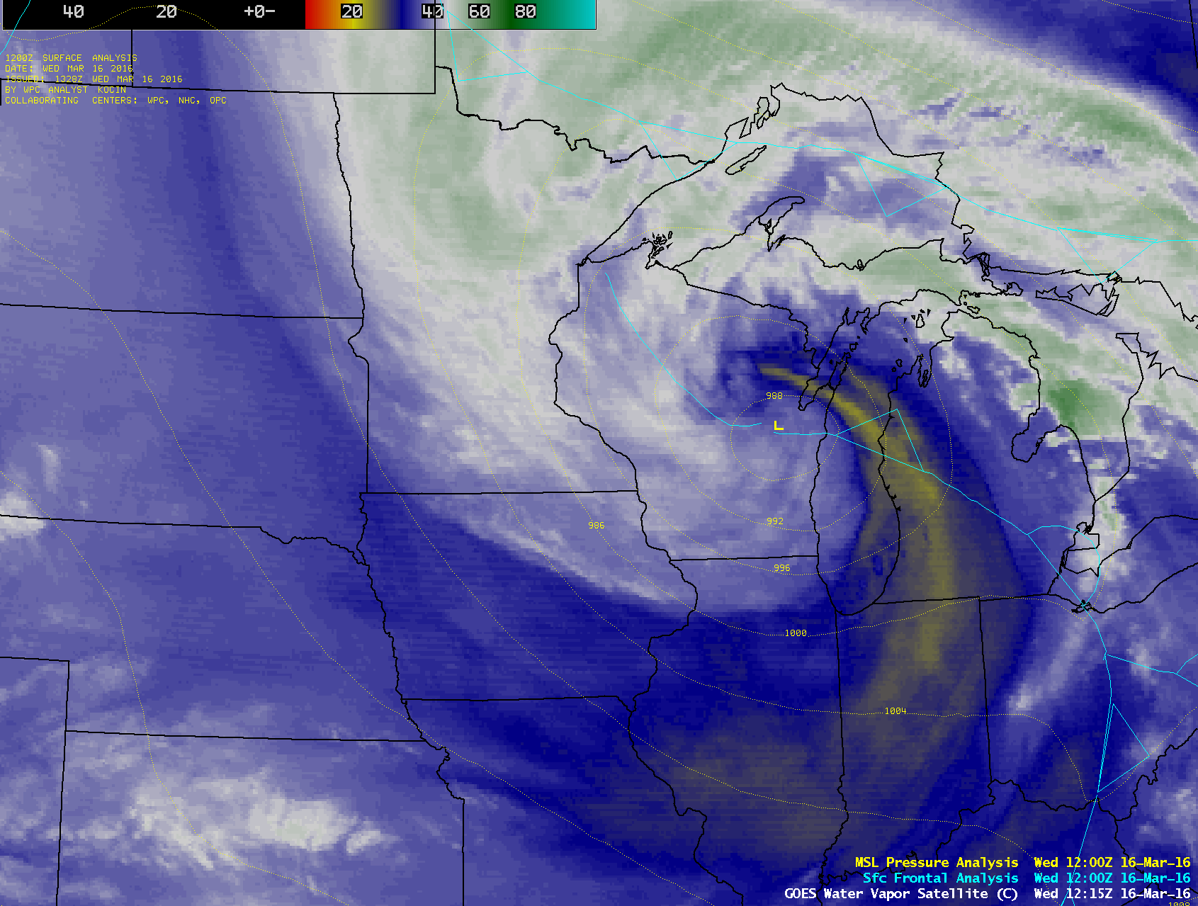
![GOES-13 Water Vapor (6.5 µm) images, with surface analyses [click to play animation]](https://cimss.ssec.wisc.edu/satellite-blog/wp-content/uploads/sites/5/2016/03/160316_goes13_water_vapor_surface_analysis_anim.gif)
![GOES-13 Visible (0.63 µm) images [click to play animation]](https://cimss.ssec.wisc.edu/satellite-blog/wp-content/uploads/sites/5/2016/03/160316_goes13_visible_metars_anim.gif)
![GOES-13 Water Vapor (6.5 µm) image, with pilot report of severe turbulence [click to enlarge]](https://cimss.ssec.wisc.edu/satellite-blog/wp-content/uploads/sites/5/2016/03/160316_0200utc_goes13_water_vapor_metars_pireps.jpg)
![GOES-13 Water Vapor image, with pilot report of severe turbulence [click to enlarge]](https://cimss.ssec.wisc.edu/satellite-blog/wp-content/uploads/sites/5/2016/03/160316_2345utc_goes13_metars_pireps.jpg)
![GOES-13 Water Vapor (6.7 µm) images with Pilot Reports of turbulence [click to play animation]](https://cimss.ssec.wisc.edu/satellite-blog/wp-content/uploads/sites/5/2016/03/160311_goes13_water_vapor_pireps_anim.gif)
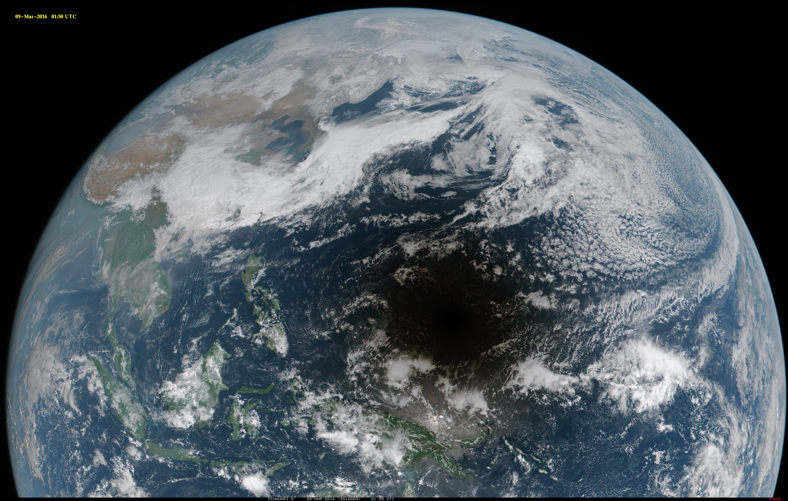
![Himawari-8 true-color images [click to play MP4 animation]](https://cimss.ssec.wisc.edu/satellite-blog/wp-content/uploads/sites/5/2016/03/1750x2750_AHIM08_B1_NHS_2016069_015000.GIF)
![COMS-1 Visible (0.67 um) images [click to play animation]](https://cimss.ssec.wisc.edu/satellite-blog/wp-content/uploads/sites/5/2016/03/160308-09_coms1_visible_solar_eclipse_shadow_anim.gif)
![GOES-15 Visible (0.63 um) images [click to play animation]](https://cimss.ssec.wisc.edu/satellite-blog/wp-content/uploads/sites/5/2016/03/160309_goes15_visible_solar_eclipse_shadow_anim.gif)
![FY-2E Visible (0.73 µm) images [click to enlarge]](https://cimss.ssec.wisc.edu/satellite-blog/wp-content/uploads/sites/5/2016/03/160309_fy2e_visible_solar_eclipse_shadow_anim.gif)
![FY-2G Visible (0.73 µm) images [click to enlarge]](https://cimss.ssec.wisc.edu/satellite-blog/wp-content/uploads/sites/5/2016/03/160309_fy2g_visible_solar_eclipse_shadow_anim.gif)
![GOES-13 Water Vapor (6.5 µm) images [click to play MP4 animation]](https://cimss.ssec.wisc.edu/satellite-blog/wp-content/uploads/sites/5/2016/03/960x1280_EASTL_B3_GOES13_WV_EAST_US_STORM_04MAR_2016064_213000_0001PANEL.GIF)
![Aqua MODIS Water Vapor (6.7 µm), Infrared (11.0 µm), and Visible (0.65 µm) images [click to enlarge]](https://cimss.ssec.wisc.edu/satellite-blog/wp-content/uploads/sites/5/2016/03/160304_1737utc_aqua_modis_water_vapor_infrared_visible_anim.gif)
![Suomi NPP VIIRS Visible (0.64 µm) and Infrared (11.45 µm) images [click to enlarge]](https://cimss.ssec.wisc.edu/satellite-blog/wp-content/uploads/sites/5/2016/03/160304_1722utc_suomi_npp_viirs_visible_infrared_anim.gif)
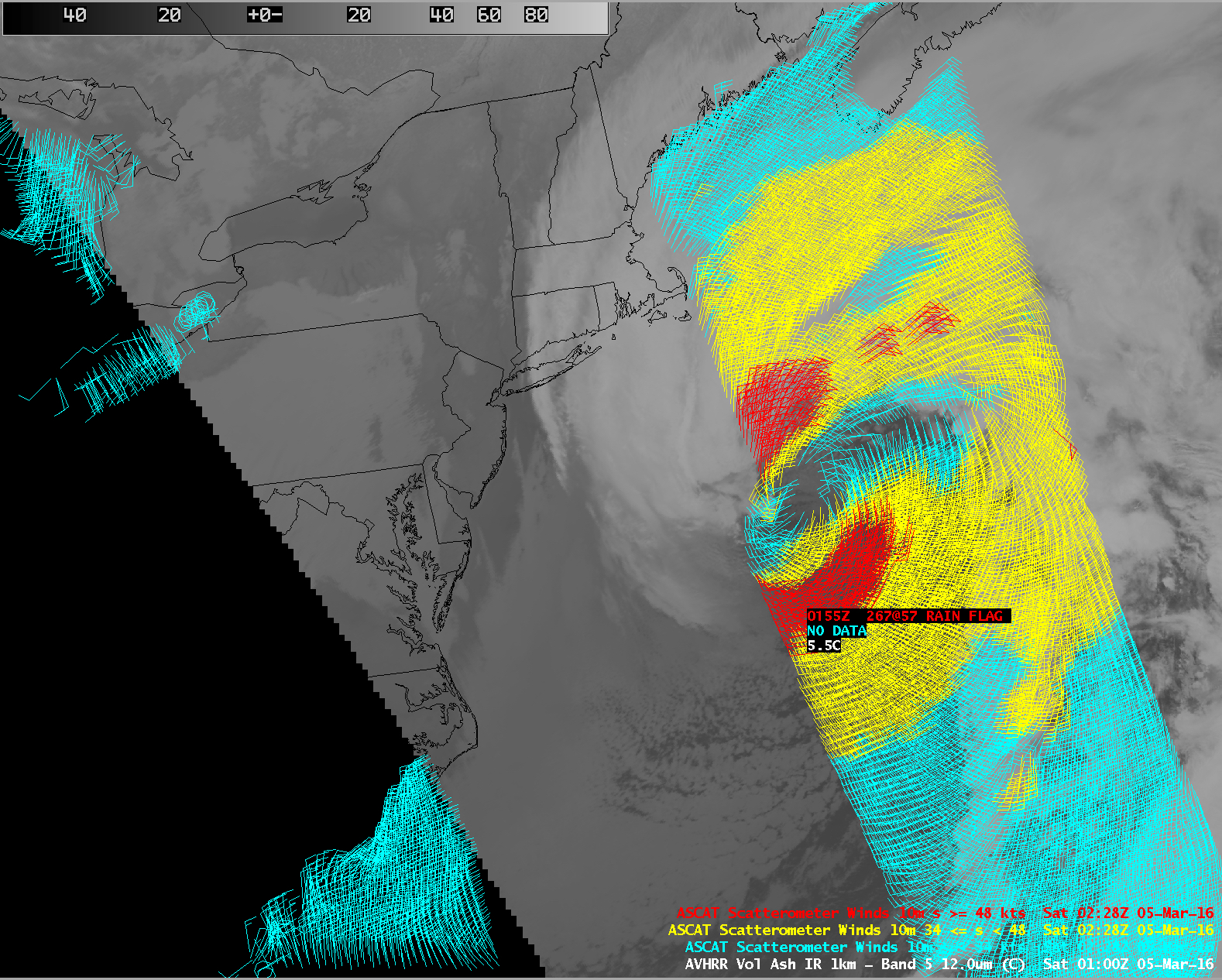
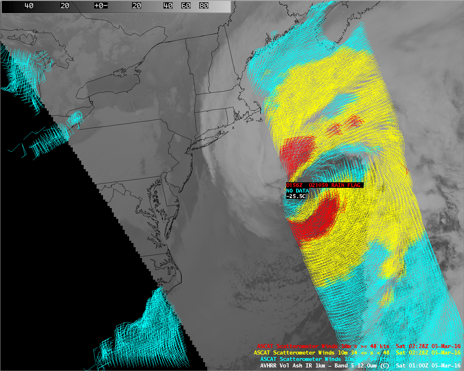
![POES AVHRR Infrared (12.0 µm) images at 1852, 2205, and 0100 UTC, with Metop ASCAT winds at 0155 UTC [click to enlarge]](https://cimss.ssec.wisc.edu/satellite-blog/wp-content/uploads/sites/5/2016/03/160304-05_poes_avhrr_infrared_ascat_anim.gif)
