This website works best with a newer web browser such as Chrome, Firefox, Safari or Microsoft Edge. Internet Explorer is not supported by this website.

Atmospheric spectra over the west Pacific

When Himawari-10 launches (currently scheduled for late 2028/early 2029), it will carry the GHMS, the Geostationary HiMawari Sounder, planned to give hourly sounder imagery (with more frequent observations — about 4 per hour — in smaller targetable domains, including one over Japan.) The Sounder will observe with about 4-km spatial resolution... Read More

When Himawari-10 launches (currently scheduled for late 2028/early 2029), it will carry the GHMS, the Geostationary HiMawari Sounder, planned to give hourly sounder imagery (with more frequent observations — about 4 per hour — in smaller targetable domains, including one over Japan.) The Sounder will observe with about 4-km spatial resolution within two spectral ranges, 4.44 µm – 5.92 µm and 9.13 µm – 14.7 µm. (The information above comes from this presentation). That spectral resolution is similar to the midwave/longwave converage on the CrIS instrument that flies on JPSS Satellites NOAA-20/NOAA-21 and Suomi-NPP. This blog post, the first in a series, shows spectra from CrIS and relates it to the observed atmosphere as a way of preparing National Weather Service staff in the Guam office to use the data. (CrIS data are downloaded in real time at the Direct Broadcast antenna at the Guam Office).

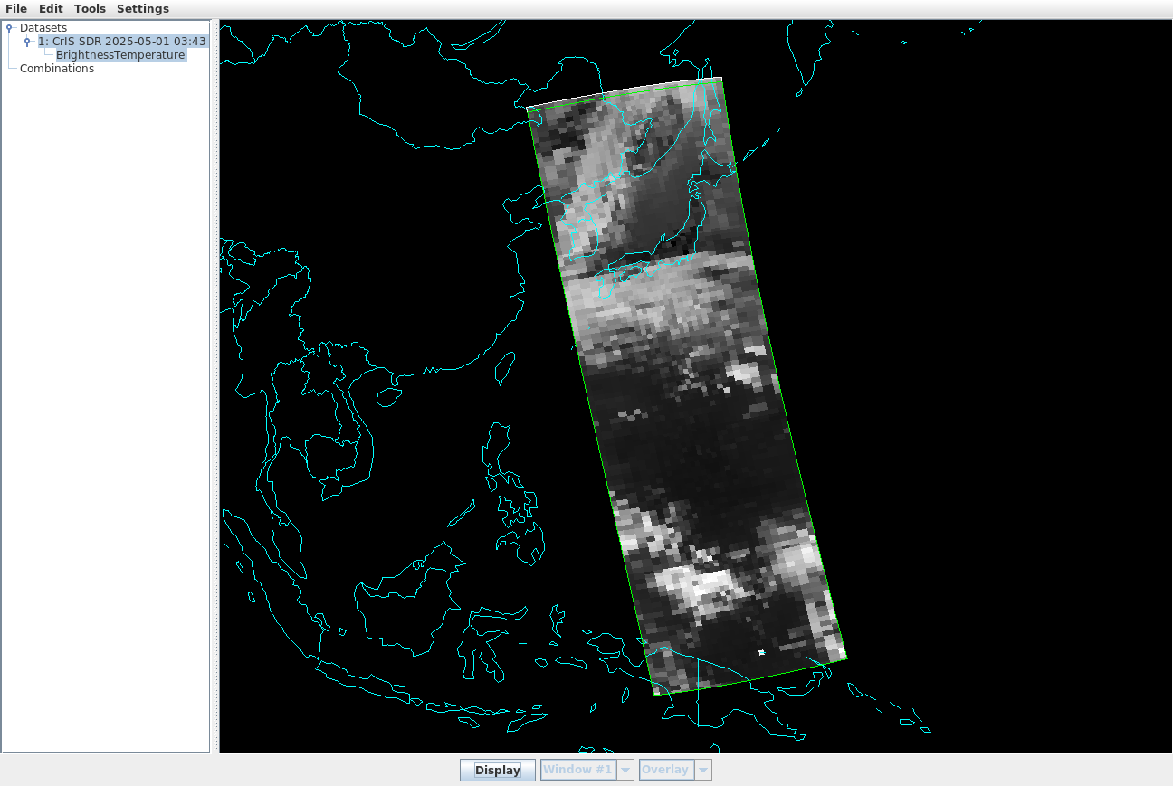
On 1 May 2025, NOAA-20 overflew the Marianas Islands at around 0350 UTC. Following the steps outlined in this blog post, NOAA-20 CrIS data were ordered from the NOAA CLASS site (here’s the list of files; Hydra expects the CrIS data — ‘SCRIF’ — and geolocation data — ‘GCRSO’ — to be combined) and were uploaded into a version of McIDAS-V that can read and interpret CrIS files. The swath loaded is shown below with the Hydra window spawned by McIDAS-V. Note the ‘Display’ button at the bottom of this window.

CrIS display within the Hydra window, data from 0343-0359 UTC on 1 May 2025 (Click to enlarge)

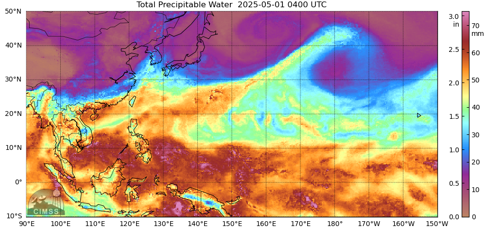
What did other satellite data show over the region? MIMIC Total Precipitable Water (TPW) fields (from this source), below, show relatively dry air around Japan and over the central Pacific between 10o and 20oN.

Total Precipitable Water fields, 0400 UTC on 1 May 2025 (Click to enlarge)

I also used geo2grid software applied to Himawari Standard Data (HSD) files and created the True Color and airmass RGB images below. The relative dryness in a longitudinal strip through Guam is apparent, as are the more moist regions to the north and south.

Himawari-9 True Color and airmass RGB over the western Pacific, 0400 UTC on 1 May 2025 (click to enlarge)

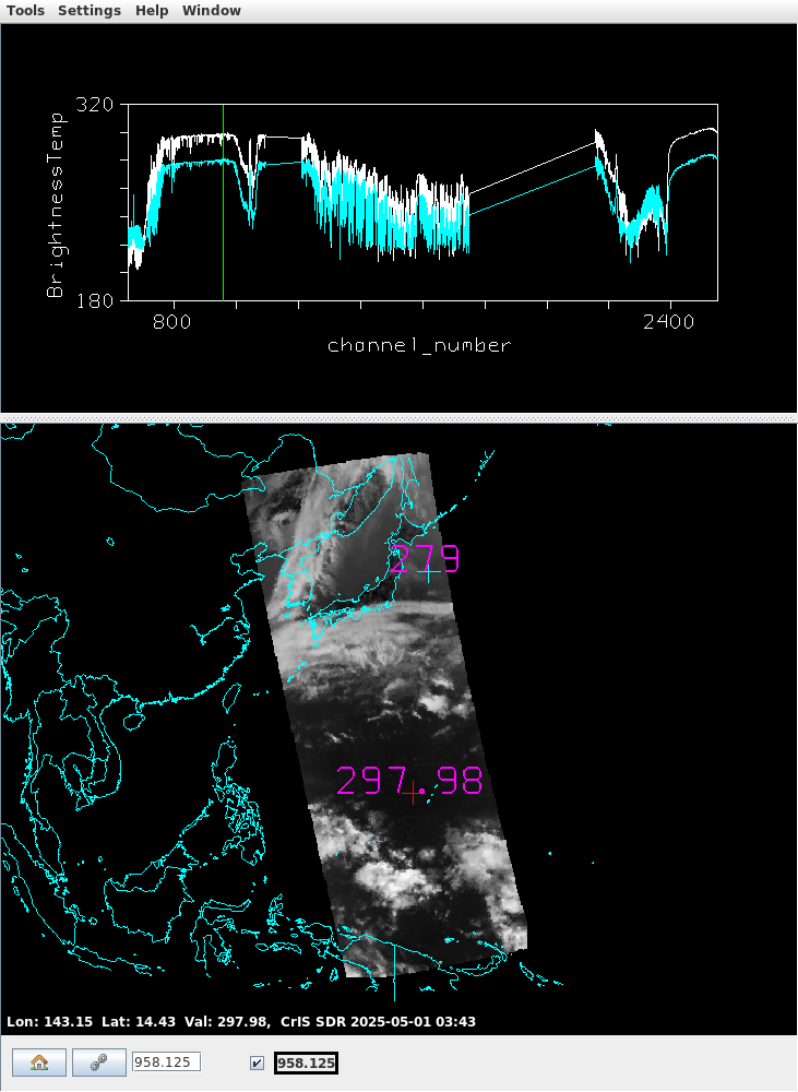
Now that you have a gross understanding of the atmosphere in this region, what do you expect the spectra to look like over this region? Clicking that ‘Display’ button in the McIDAS-V Hydra window spawns an interactive window, two examples of which are shown below. Two spectra are shown: the cyan spectra is derived from data at the northernmost point, showed over Japan; the white spectra is derived from data closer to Guam. The horizontal mapping of data in the images on the bottom in the figures is at the wavenumber that matches the vertical green line, i.e., wavenumber 828.75 (equivalent to 12.07 µm) on the left and 958.125 (equivalent to 10.44 µm) on the right. The wavenumber to wavelength conversion was done here.

Atmospheric Spectra at two locations (as indicated by crosses on the map); the greyscale values (and probe values) on the bottom match the location of the green vertical line in the spectra above. A wavenumber of 828.75 is 12.07 µm; 958.125 is 10.44 µm ; note that the channel number increment along the x-axis is 200.

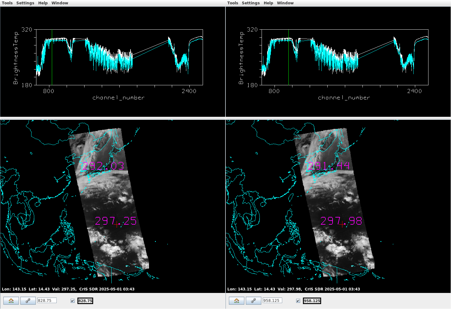
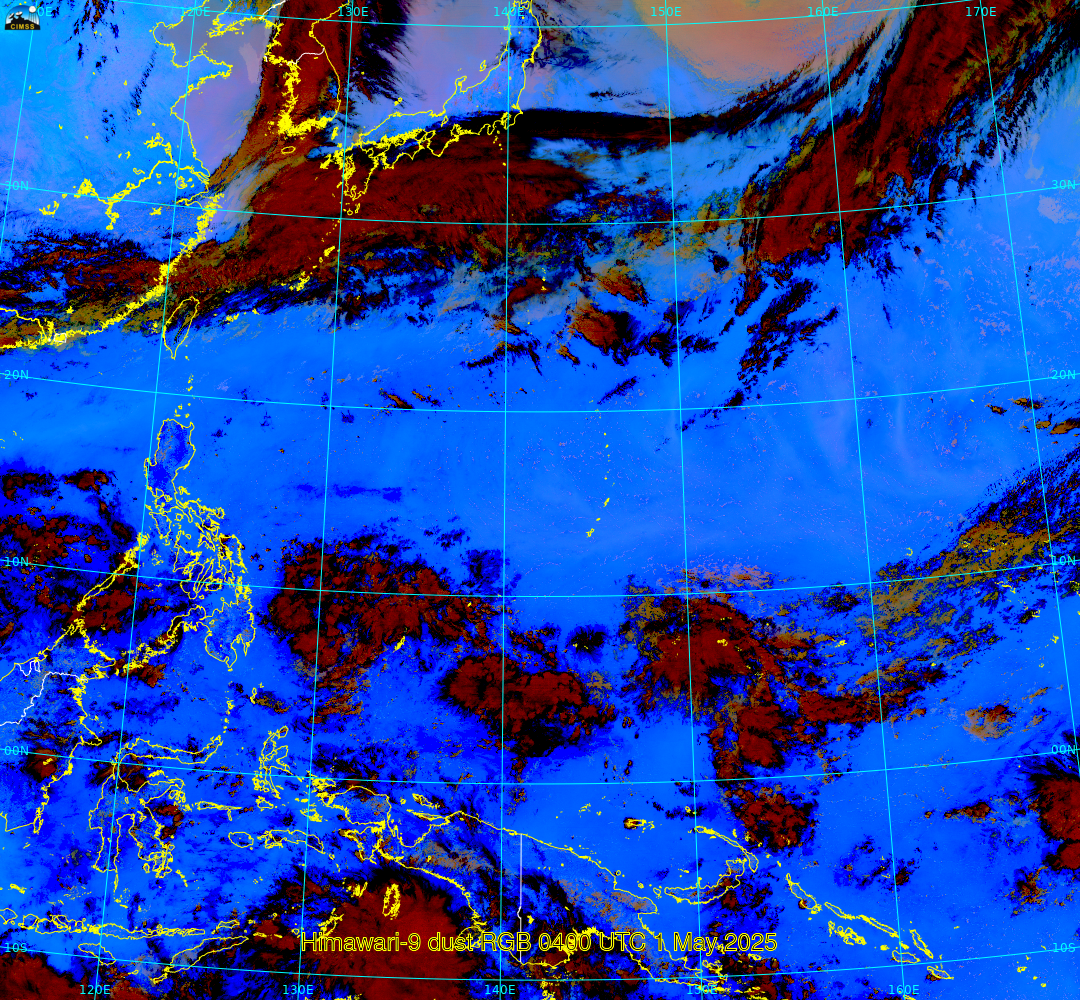
What can you infer from those spectra at the two different points? Note first the strong cooling where ozone absorption is present at wavenumbers around 1050. Wavenumbers exceeding 2200 — the shortwave part of the electromagnetic spectrum — are not slated to be observed by GHMS. Pay attention to the slope of the two spectra between 800 and 1000; in the white line, brightness temperature change more over the range over Guam — the white line — compared to over Japan — the cyan line. Brightness temperature differences plotted at the points on the map over Guam are 297.98 K in the clean window at 10.44 µm and 297.25 K in dirty window at 12.07 µm, for a difference of 0.73 K and over Japan are 291.44 K in the clean window (10.44 µm) and 292.03 (12.07 µm), for a difference of -0.59K! (Editors note: I was not expecting this, and when I saw that, my reaction was to create the dust RGB below) The negative difference suggest the presence of dust and the dust RGB shows a pinkish hue around Japan, a color in that RGB that is consistent with dust. You can infer something about the atmosphere from the slope of the the spectrum between wavenumbers 830 and 960. If it shows increasing temperatures, i.e., warming, then the atmosphere is likely moist. If it shows level or decreasing brightness temperatures, maybe dust is present.

Himawari-9 dust RGB, 0400 UTC on 1 May 2025 (Click to enlarge)

In the spectrum below, the northern point has been moved out of the region where the dust RGB suggests dust is present. The slope of the cyan spectra shows warming brightness temperatures from wavenumbers 800 to 980 is consistent with a decrease of water vapor absorption as observations move from the dirty window to the clean window in the infrared spectrum.

Atmospheric Spectra at two locations (as indicated by crosses on the map); the greyscale values (and probe values) on the bottom match the location of the green vertical line in the spectra above. The plot below shows brightness temperatures at wavenumber of 958.125 is 10.44 µm ; the channel number increment along the x-axis is 200.

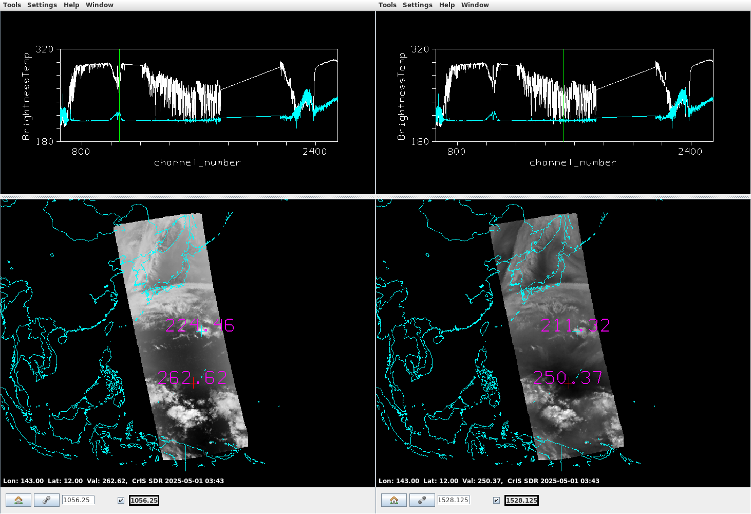
Two different points are examined in the plots below. The greyscale plot on the left is wavenumber 1056.25 (or 9.46 µm, in a region of ozone absorption) and the one of the right is 1528.125 (or 6.5 µm, a region of water vapor absorption). The cyan spectra corresponds to the point centered over convection; the white spectra is in the warmest region at 6.5 µm. The cyan spectrum — a region of cloudiness, as the ‘+’ is centered over a convective cloud — is (mostly) uniformly cold except in the Ozone Absorption band where the spectra shows a local maximum in brightness temperature, and in the shortwave infrared (wavenumbers around 2400 are at 4) where solar radiation is present and in the longwave (wavenumbers around 750 are at 13.3) where CO2 absorption will have an effect. In the white spectrum, at a point in clear air, ozone absorption does not have a warming effect, and the large valley of variable water vapor absorption from wavenumbers 1200-1600 is apparent. In addition, surface features are not discernible at these wavenumbers unlike in the window channels (wavenumbers 828 and 958) shown above.

Atmospheric Spectra at two locations (as indicated by crosses on the map); the greyscale values (and probe values) on the bottom match the location of the green vertical line in the spectra above. A wavenumber of 1056.25 (left) is 9.46 µm; 1528.125 is 6.5 µm ; the channel number increment along the x-axis is 200.

This is the first of several posts on this topic. Stay tuned!

View only this post Read Less

Persistent convection over Tutuila, American Samoa late on 30 April Samoa Standard Time

GOES-18 imagery/products, shown below, depict an area of enhanced instability and moisture centered on American Samoa, and convection develops and persists over/around the main island of American Samoa, Tutuila. The convection appears to form along an east-west line that drifts over the island between 0400 and 0800 UTC.Total Precipitable Water... Read More

GOES-18 imagery/products, shown below, depict an area of enhanced instability and moisture centered on American Samoa, and convection develops and persists over/around the main island of American Samoa, Tutuila. The convection appears to form along an east-west line that drifts over the island between 0400 and 0800 UTC.

GOES-18 Derived Lifted Index (in clear air, scaled from -5 to 5) and Clean Window infrared (Band 13, 10.3) imagery, 0300 – 0950 UTC on 1 May 2025 (Click to enlarge)

Total Precipitable Water fields, below, suggest the convection was at the leading edge of a somewhat more moist airmass: TPWs increased from 1.8″ (reddish in the enhancement) to 2.0+” (lilac/purple in the enhancement) as the convection developed on the leading edge of the enhanced moisture.

GOES-18 Derived Total Precipitable Water (in clear air) and Clean Window infrared (Band 13, 10.3) imagery, 0300 – 0950 UTC on 1 May 2025 (Click to enlarge)

CSPP Geosphere visible/night microphysics RGB imagery, below, (click here for a faster animation, also from 0010 – 1210 UTC on 1 May 2025) shows the progression of the convection from low-level clouds to strong showers. The low-level outflow boundaries show up nicely as light blue/white/pink arcs that become progressively more dark red as the convection develops.

GOES-18 Full DIsk imagery, 0010 UTC – 1210 UTC on 1 May 2025

What other products are useful in diagnosing the atmosphere? The SSEC/CIMSS Tropical Weather page includes wind diagnostics over the South Pacific, and they can be retrieved from the data archive at that page. The vorticity analysis from 21 UTC/30 April 2025 to 120 UTC/1 May 2025, below, shows an increase in low-level vorticity over Samoa, reflecting the convective development that is occurring there. The center of the vorticity slowly drifts north as well during the animation. The vorticity fields have a structure that is in agreement with the observed convection; however, upper-level divergence and low-level convergence fields (not shown) do not.

Diagnosed 850-mb vorticity from 2100 UTC on 30 April through 1200 UTC on 1 May 2025 (Click to enlarge)

MIMIC Total Precipitable Water fields (source), below, also show the subtle increase in TPW that accompanied the convection over Samoa.

Hourly MIMIC Total Precipitable Water fields over the South Pacific, 2000 UTC 30 April – 1200 UTC 1 May 2025 (Click to enlarge)

Scatterometry data for this event was sparse. The toggle below — images that were taken from the manati website (https://manati.star.nesdis.noaa.gov/) — shows OSCAT imagery at 1128 UTC and MetopC imagery at 2013 UTC (both on 30 April 2025). There is speed convergence to the southeast of American Samoa.

OSCAT-3 (1128 UTC) and MetopC ASCAT (2013 UTC) scatterometery on 30 April 2025 (Click to enlarge)

LightningCast probabilities (available from an American Samoa Sector at this website) shows increasing probabilities from 0300 UTC to 0600 UTC, with GLM lightning observations starting at 0440 UTC.

LightningCast probabilities, 0300 – 0600 UTC plotted over GOES-18 clean window infrared imagery, along with GLM observations of Flash Extent Density, 1 May 2025 (Click to enlarge)

LightningCast probabilities can also be calculated with CSPP Geo software, and the output for a longer period is shown below.

LightningCast Probability, 0000 – 1000 UTC on 1 May 2025 (Click to enlarge) ; the underlying satellite imagery changes at 0440 UTC, around sunset

NUCAPS profiles can give a good estimate of the thermodynamic state of the atmosphere. Gridded NUCAPS fields, not shown here, are very useful because they show horizontal fields that allow for a quicker diagnostic of thermodynamics than via the tedious clicking of multiple sounding points. These profiles can be compared to the 0000 UTC/1200 UTC 1 May 2025upper-air sounding from the balloon launched from the Pago Pago airport, shown below. These plots were retrieved from the University of Wyoming sounding site.

Upper air sounding at NSTU/91765 0000 and 1200 UTC 1 May 2025 (Click to enlarge)

What did the NUCAPS profiles show? NUCAPS Sounding availability at 0008 UTC (NOAA-20) and 0059 UTC (NOAA-21) are shown below.

NUCAPS Sounding Availability at 0008 and 0059 UTC on 1 May 2025 (Click to enlarge)

The four closest profiles to Tutuila, shown in the animation below, all have similar thermodynamic characteristics. Moisture is more abundant in the easternmost points.

NUCAPS Sounding Availability, and Profiles/Diagnosed information for the 4 points closest to Tutuila, 0018 UTC on 1 May 2025 (Click to enlarge)

The information from NOAA-21, at 0058 UTC, below, along a north-south line that passes north-south through the diagnosed maximum in instability, shows CAPE values are greatest just north of the American Samoa islands, and Total Precipitable Water is greatest over the islands.

NUCAPS profiles along a North-South line to the east of Tutuila, as indicated; profiles are at 0108 UTC on 1 May 2025 (Click to enlarge)

View only this post Read Less

Strong winds across Pennsylvania

Storm Prediction Center storm reports for the 24 hours ending 1200 UTC on 30 April 2025 show a line of strong wind reports from the mid-Mississippi River valley east-northeastward into central Pennsylvania. What satellite products could have been useful on 29 April to anticipate the arrival of these strong winds?... Read More

Storm Prediction Center storm reports for the 24 hours ending 1200 UTC on 30 April 2025 show a line of strong wind reports from the mid-Mississippi River valley east-northeastward into central Pennsylvania.

SPC Storm Reports for the 24 hours ending 1200 UTC on 30 April 2025

What satellite products could have been useful on 29 April to anticipate the arrival of these strong winds? The animation below shows Derived Lifted Index (a clear-sky only product) values plotted on top of visible imagery. Lifted Index values between -2 and -5 are widespread through much of the animation over western Pennsylvania. Convection moving in from the west will be able to access this instability.

GOES-East visible imagery (Band 2, 0.64 µm) and Derived Lifted Index (scaled from -5 to 10), 1441 UTC on 29 April 2025 to 0001 UTC on 30 April 2025 (Click to enlarge)

NUCAPS profiles were also available over Pennsylvania in a cluster from 1500-1800 UTC, as shown in the animation below. The ‘Sounding Availability Plot’ includes more than one overpass, and selected profiles are shown over central Pennsylvania. Of particular note is the region in very rural Clearfield County where three profiles were sensed over the course of 3 hours! It’s worth repeating that the NUCAPS points are actually a volume of air, a tube about 50km in diameter that matches the ATMS footprint. Considerable destabilization is diagnosed over the three hours. Based on these profiles, a forecaster observing the severe weather reports upstream might not suspect that incoming convection will weaken. (Here’s an animation of just the three profiles over rural Clearfield County).

NUCAPS Profiles over central Pennsylvania, 1500-1800 UTC on 29 April 2025 (Click to enlarge)

Clean window infrared imagery, below, spanning from 1900 UTC on 29 April through 0300 UTC on 30 April 2025, shows that coldest cloud tops warmed as the convection moved into central Pennsylvania. However, widespread power outages were reported, as shown here from this source.

GOES-19 Clean Window infrared (Band 13, 10.3 µm) imagery, 1900 UTC/29 April 2025 – 0300 UTC/30 April 2025

Were the power outages caused by the storms visible in the Day Night band, similar to this event in Spain? The toggle below compares Day Night Band imagery from early morning on the 29th (before the storms) and early morning on the 30th (just after the storms). It’s hard to tell for sure because a lot of the changes in illumination on 30 April are due to the thick cloud cover from the storms.

Day Night Band imagery over Pennsylvania, 0636 UTC on 29 April and 0758 UTC on 30 April 2025 (Click to enlarge)

View only this post Read Less

Giant hail and damaging winds in Texas

1-minute Mesoscale Domain Sector GOES-19 (GOES-East) “Red” Visible (0.64 µm) and “Clean” Infrared Window (10.3 µm) images (above) showed thunderstorms that produced giant hail (as large as 5.00 inches in diameter) and damaging wind gusts (as high as 106 mph) across the Texas Panhandle and North Texas (SPC Storm Reports) on 29 April 2025. The Infrared images revealed pulses of... Read More

1-minute GOES-19 “Red” Visible (0.64 µm, top) and “Clean” Infrared Window (10.3 µm, bottom) images with time-matched (+/- 3 minutes) SPC Storm Reports plotted in red/white, from 1920 UTC on 29 April to 0010 UTC on 30 April [click to play animated GIF | MP4]

1-minute Mesoscale Domain Sector GOES-19 (GOES-East) “Red” Visible (0.64 µm) and “Clean” Infrared Window (10.3 µm) images (above) showed thunderstorms that produced giant hail (as large as 5.00 inches in diameter) and damaging wind gusts (as high as 106 mph) across the Texas Panhandle and North Texas (SPC Storm Reports) on 29 April 2025. The Infrared images revealed pulses of thunderstorm overshooting tops that exhibited 10.3 µm brightness temperatures as cold as -78ºC (brighter white pixels embedded within dark black regions) — and the signature of an Above-Anvil Cirrus Plume (reference) was evident in Visible imagery (although the warmer AACP signature was less distinct in the lower-resolution Infrared images).

According to a plot of rawinsonde data (source) from Fort Worth, Texas at 0000 UTC on 30 April (below), the coldest GOES-19 cloud-top infrared brightness temperature of -78ºC represented a ~1.5 km overshoot of the Most Unstable air parcel Equilibrium Level (MU EL).

Plot of rawinsonde data from Fort Worth, Texas at 0000 UTC on 30 April [click to enlarge]

GOES-19 Visible images with plots of GLM Flash Points (below) displayed abundant lightning activity associated with these supercell thunderstorms — which were generally focused in the vicinity of a quasi-stationary frontal boundary.

1-minute GOES-19 Visible (0.64 µm) images with plots of 1-minute GOES-19 GLM Flash Points, from 1910 UTC on 29 April to 0009 UTC on 30 April [click to play MP4 animation]

View only this post Read Less