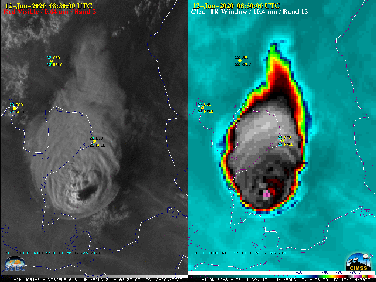
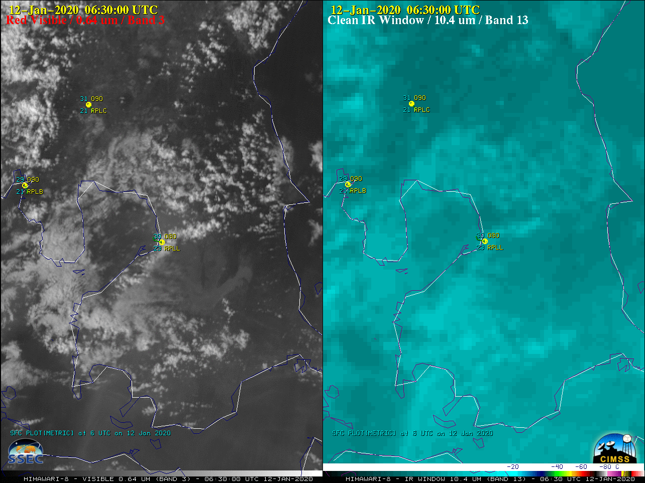
Himawari-8 “Red” Visible (0.64 µm, left) and “Clean” Infrared Window (10.4 µm, right) images [click to play animation | MP4]
![Himawari-8 "Red" Visible (0.64 µm) and "Clean" Infrared Window (10.4 µm) images at 1910 UTC [click to enlarge]](https://cimss.ssec.wisc.edu/satellite-blog/images/2020/01/200112_0910utc_himawari8_visible_infrared_Tall_anim.gif)
Himawari-8 “Red” Visible (0.64 µm) and “Clean” Infrared Window (10.4 µm) images at 1910 UTC [click to enlarge]
![Plots of rawinsonde data from Legaspi, Mactan and Laoag in the Philippines [click to enlarge]](https://cimss.ssec.wisc.edu/satellite-blog/images/2020/01/200112_RPMP_RPMT_RPLI_raobs_anim.gif)
Plots of rawinsonde data from Legaspi, Mactan and Laoag in the Philippines [click to enlarge]
The TROPOMI detected SO2 at altitude of 20km on 13 January:
The SO2 signal from #Taal detected by #TROPOMI on 2020-01-13 has an altitude of up to 20km. #SO2LH. @tropomi @DLR_en @ESA_EO pic.twitter.com/x6nstNRWUw
— TROPOMI SO2 (@DlrSo2) January 13, 2020
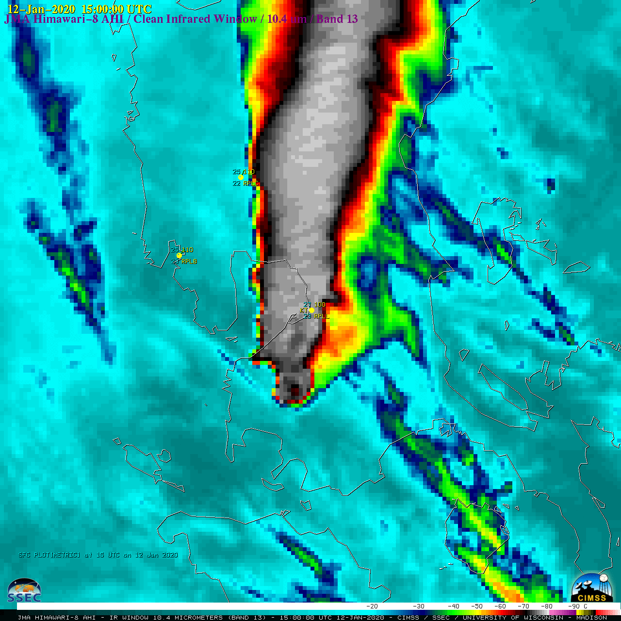
A longer animation of Himawari-8 Infrared imagery revealed the intermittent presence of the warm wake feature until about 1400 UTC. The coldest 10.4 µm cloud-top brightness temperature was -89.7ºC.
![Himawari-8 "Clean" Infrared Window (10.4 µm) images [click to play animation | MP4]](https://cimss.ssec.wisc.edu/satellite-blog/images/2020/01/200112_himawari8_infrared_zoom_Taal_anim.gif)
Himawari-8 “Clean” Infrared Window (10.4 µm) images [click to play animation | MP4]
![Himawari-8 "Clean" Infrared Window (10.4 µm) images [click to play animation | MP4]](https://cimss.ssec.wisc.edu/satellite-blog/images/2020/01/200112_himawari8_infrared_Taal_anim.gif)
Himawari-8 “Clean” Infrared Window (10.4 µm) images [click to play animation | MP4]
![NOAA-20 VIIRS Day/Night Band (0.7 µm) and Infrared Window (11.45 µm) images at 1648 UTC (credit: William Straka, CIMSS) [click to enlarge]](https://cimss.ssec.wisc.edu/satellite-blog/images/2020/01/200112_1648utc_noaa20_viirs_dayNightBand_infraredWindow_Taal_anim.gif)
NOAA-20 VIIRS Day/Night Band (0.7 µm) and Infrared Window (11.45 µm) images at 1648 UTC (credit: William Straka, CIMSS) [click to enlarge]
![Split Window Difference (11-12 um) images from Terra MODIS, NOAA-20 VIIRS and Suomi NPP VIIRS [click to enlarge]](https://cimss.ssec.wisc.edu/satellite-blog/images/2020/01/200112_modis_viirs_splitWindowDifference_Taal_anim.gif)
Split Window Difference (11-12 µm) images from Terra MODIS, NOAA-20 VIIRS and Suomi NPP VIIRS [click to enlarge]
#TaalEruption as seen from @VaisalaGroup merged total lightning (NLDN and GLD) 15-min plots. This lapse is about 15 hours long and lightning activity has quieted since. ?#TaalEruption2020 #TaalVolcano @COweatherman pic.twitter.com/kkxjztq9KU
— William Churchill (@kudrios) January 13, 2020
Volcanic eruption at #TaalVolcano with AMAZING #volcano #lightning display. Remind me later to get counts. Data from @VaisalaGroup #GLD360. #VaisalaDigital #AMS2020 @janinekrippner @C_MarieSmith @volcaniclastic @simoncarn @CorCima pic.twitter.com/vYpgPJRoGC
— Ch?is Vagas|?y (@COweatherman) January 12, 2020
If you’re mesmerized by the steamy #Taal eruption plume and wondering why it’s creating so much #VolcanicLightning, you’re not alone. Here’s a micro-crash course on the physics of volcanic thunderstorms for non-specialists. Thanks to @joshibob_ for the incredible footage! (1/14) pic.twitter.com/CCl6zw56RZ
— Alexa Van Eaton (@volcaniclastic) January 13, 2020
===== 14 January Update =====
![GOES-17 SO2 RGB images [click to play animation | MP4]](https://cimss.ssec.wisc.edu/satellite-blog/images/2020/01/200114_goes17_so2RGB_Taal_anim.gif)
GOES-17 SO2 RGB images [click to play animation | MP4]
Volcanic SO2 cloud from #TaalVolcano is moving further East towards Alaska. #TROPOMI @TROPOMI @Sentinel5p @ESA_EO @DLR_en @BIRA_IASB #SO2LH pic.twitter.com/Brp4Iig0PV
— TROPOMI SO2 (@DlrSo2) January 14, 2020
View only this post Read Less
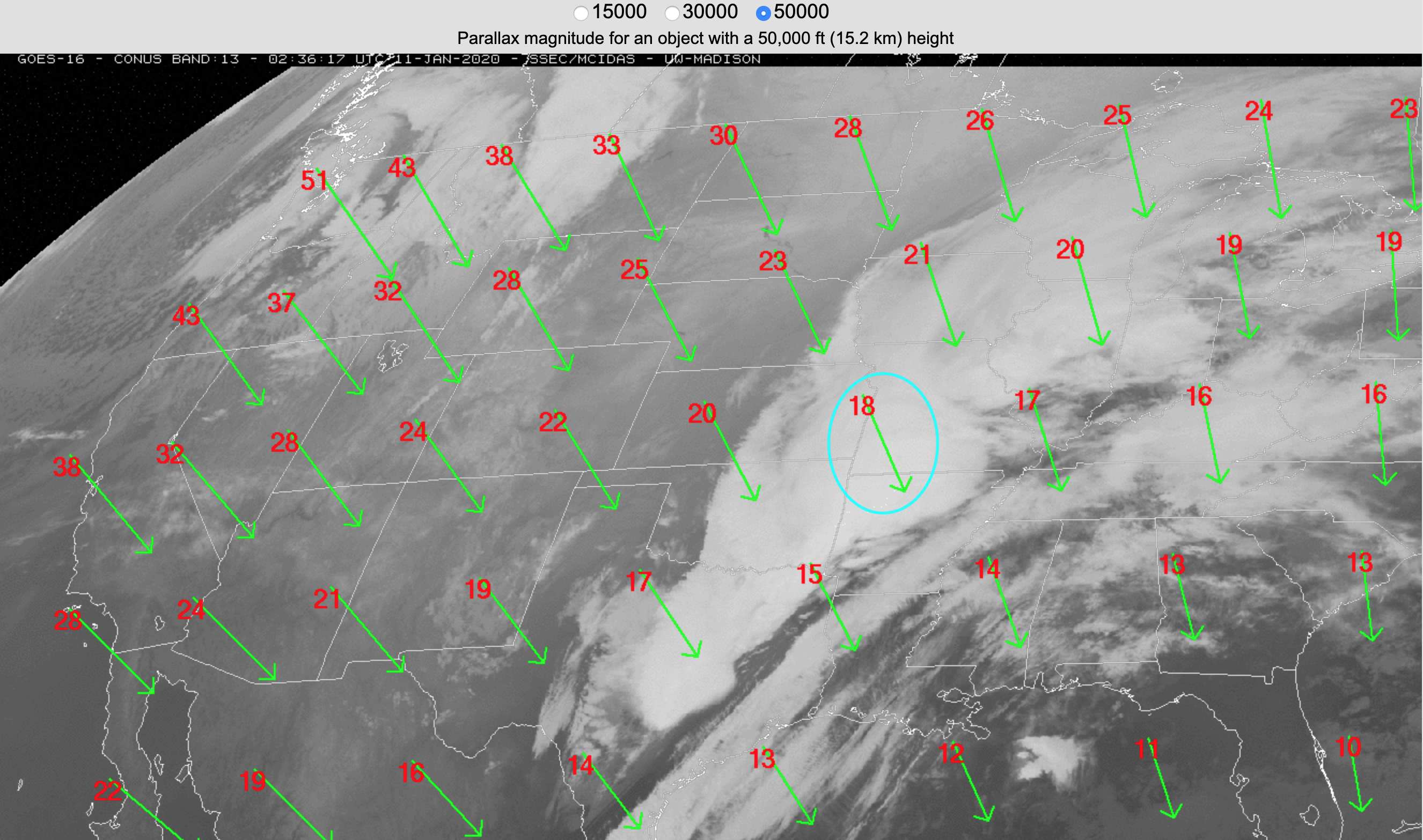
![GOES-16 "Red" Visible (0.64 µm) images, including plot of SPC Storm Reports (with and without parallax correction) [click to play animation]](https://cimss.ssec.wisc.edu/satellite-blog/images/2020/01/200110_goes16_visible_spcStormReports_parallax_KS_MO_OK_AR_anim.gif)
![GOES-16 "Red" Visible (0.64 µm) image at 2030 UTC, including plot of SPC Storm Reports (with and without parallax correction) [click to enlarge]](https://cimss.ssec.wisc.edu/satellite-blog/images/2020/01/200110_2030utc_goes16_visible_spcStormReport_parallax_anim.gif)
![GOES-16 "Red" Visible (0.64 µm) image at 2051 UTC, including plot of Tornado report (with and without parallax correction) [click to enlarge]](https://cimss.ssec.wisc.edu/satellite-blog/images/2020/01/200110_2051utc_goes16_visible_spcStormReport_parallax_anim.gif)
![GOES-16 parallax direction vectors and magnitude (km) for a cloud top feature at 15 km [click to enlarge]](https://cimss.ssec.wisc.edu/satellite-blog/images/2020/01/200110_KS_MO_parallax.png)
![GOES-17 parallax correction direction vectors and magnitude (km) for a cloud top feature at 50,000 feet (15.2 km) [click to enlarge]](https://cimss.ssec.wisc.edu/satellite-blog/images/2020/01/goes17_parallax_fulldisk.png)


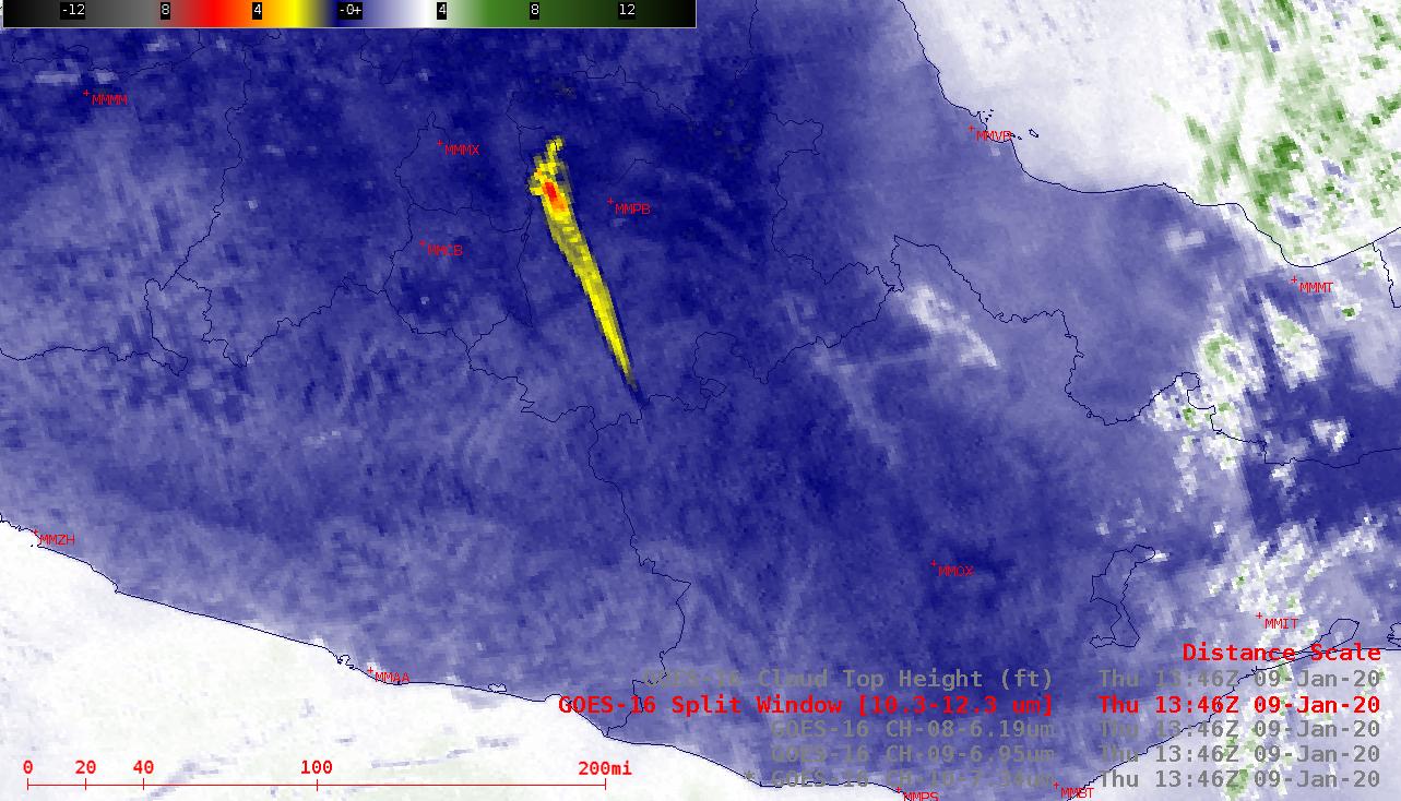
![GOES-16 Low-, Mid- and Upper-level Water Vapor (7.3 µm, 6.9 µm and 6.2 µm), Split Window Difference (10.3-12.3 µm) and Cloud Top Height product [click to play animation | MP4]](https://cimss.ssec.wisc.edu/satellite-blog/images/2020/01/200109_goes16_waterVapor_splitWindowDifference_Popocatepetl_anim.gif)
![Plots of rawinsonde data from Mexico City and Acapulco at 12 UTC [click to enlarge]](https://cimss.ssec.wisc.edu/satellite-blog/images/2020/01/200109_12UTC_MMMX_MMAA_RAOBS.GIF)
![GOES-16 Ash RGB images {click to play animation | MP4]](https://cimss.ssec.wisc.edu/satellite-blog/images/2020/01/GOES-16_RadM2_ash_2020009_140200_2020009_163000.gif)
![GOES-16 Ash Height product [click to play animation MP4]](https://cimss.ssec.wisc.edu/satellite-blog/images/2020/01/200109_ashHeight_Popocatepetl_anim.gif)
