This blog posts describes how to use NOAA’S CLASS (Comprehensive Large Array-data Stewardship System) system (link) that contains Level-2 GLM data, (under the GOES-R Series GLM L2+ Data Product (GRGLMPROD) tab) to create useable GLM imagery. GLM processing produces three Level 2 files each minute, and those files can be processed to produce imagery. First, choose... Read More
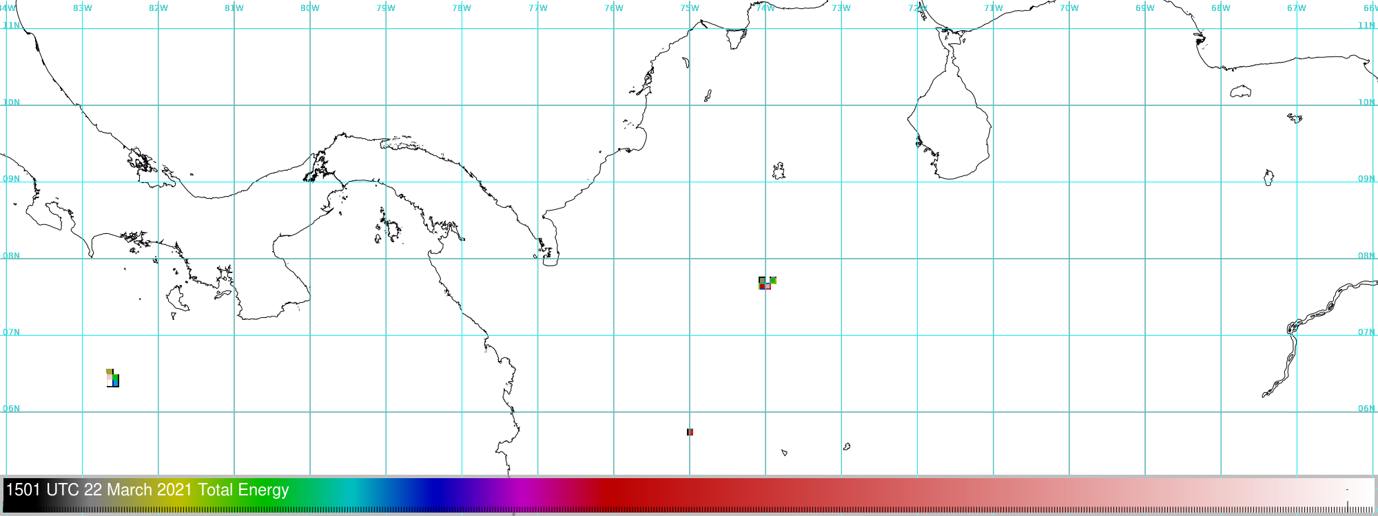
GOES-16 Gridded GLM imagery of Total Optical Energy for the 1 minute ending 1501 UTC on 22 March 2021 (Click to enlarge)
This blog posts describes how to use NOAA’S CLASS (Comprehensive Large Array-data Stewardship System) system (link) that contains Level-2 GLM data, (under the GOES-R Series GLM L2+ Data Product (GRGLMPROD) tab) to create useable GLM imagery. GLM processing produces three Level 2 files each minute, and those files can be processed to produce imagery. First, choose the time range you want in CLASS, and get the global imagery. For this blog post, I chose GOES-16 data on 22 March 2021 between 15:00 an 15:15 UTC. On the CLASS website, I clicked the GLM L2+ Lightning Detection Data and didn’t filter by any values (CLASS allows you to filter by minimum/maximum flash, event and group counts, if you want). This request returned 47 different files, but that is only about 10 Mbytes. Some of the file names — two minutes’ worth — are shown below: LCFA files from julian Day 081 (that is, 3/22/2021) starting at 15:00:00:00, 15:00:00:20, 15:00:00:40, … etc.
OR_GLM-L2-LCFA_G16_s20210811500000_e20210811500203_c20210811500218.nc

OR_GLM-L2-LCFA_G16_s20210811500200_e20210811500404_c20210811500425.nc

OR_GLM-L2-LCFA_G16_s20210811500400_e20210811501003_c20210811501016.nc

OR_GLM-L2-LCFA_G16_s20210811501000_e20210811501205_c20210811501226.nc

OR_GLM-L2-LCFA_G16_s20210811501200_e20210811501403_c20210811501419.nc
Code to convert these files (that contain raw-ish group, event and flash fields) to gridded GLM fields (that can be displayed with, for example, Geo2Grid, or AWIPS) is within the CSPP Gridded GLM software package that can be downloaded here (free registration may be required; the Gridded GLM tarball to download includes a short and useful README). To create a data file that is properly configured for Geo2Grid (or AWIPS), with software that uses the open-source glmtools software developed by Dr. Eric Bruning at Texas Tech, use this command:
cspp-geo-gglm.sh ../../data/OR_GLM-L2-LCFA_G16_s20210811501*
That will create a file with a name like this:
CG_GLM-L2-GLMF-M3_G16_s20210811501000_e20210811502000_c20210821745120.nc;
Geo2Grid can then be used to create imagery from the newly-created netCDF file. The Geo2Grid code used is below.
../p2g_grid_helper.sh TestGridded   -75.0  8. 1000 -1000 2000 750  > $GEO2GRID_HOME/TestGridded.conf

../geo2grid.sh -r glm_l2  -w geotiff -p total_energy -g TestGridded --grid-configs $GEO2GRID_HOME/TestGridded.conf --method nearest -f /home/scottl/CSPPGeo/GGLM/cspp-geo-gridded-glm-1.0b1/bin/CG_GLM-L2-GLMF-M3_G16_s20210811501000_e20210811502000_c20210821745120.nc

../add_colormap.sh ../../../enhancements/TotalEnergy.txt  GOES-16_GLM_total_energy_20210322_150100_TestGridded.tif

../add_coastlines.sh --add-coastlines --coastlines-resolution=h --coastlines-outline='black' --add-grid --grid-text-size 12 --grid-d 1.0 1.0 --grid-D 1.0 1.0  --add-colorbar --colorbar-tick-marks 250.0 --colorbar-text-size 1 --colorbar-no-ticks --colorbar-align bottom GOES-16_GLM_total_energy_20210322_150100_TestGridded.tif

convert GOES-16_GLM_total_energy_20210322_150100_TestGridded.png       -gravity Southwest -fill white -pointsize 24 -annotate +8+30 "1501 UTC 22 March 2021 Total Energy" GOES-16_GLM_total_energy_20210322_1501_Labeled.png
The Geo2Grid package commands above (1) created the grid (‘TestGridded’) onto which the data were interpolated; (2) created the imagery from the netCDF file output from the Gridded GLM package; (3) Added a pre-defined colormap (within ‘TotalEnergy.txt’); (4) Added coastlines, a lat/lon grid, and a colorbar and (5) annotated the image. This last command used ImageMagick.
Note that the GLM image created, shown at top, is mostly transparent. Three areas of GLM observations are apparent, two over South America, one over the Pacific Ocean south of Panama. The transparency is handy if you want to overlay GLM data on top of ABI imagery!
View only this post
Read Less
![Meteosat-11 Ash Height images [click to play animation | MP4]](https://cimss.ssec.wisc.edu/satellite-blog/images/2021/03/210324_meteosat11_ashHeight_Etna_anim.gif)
![Meteosat-11 Ash Loading images [click to play animation | MP4]](https://cimss.ssec.wisc.edu/satellite-blog/images/2021/03/210324_meteosat11_ashLoading_Etna_anim.gif)
![Suomi NPP VIIRS Ash Loading at 1200 UTC [click to enlarge]](https://cimss.ssec.wisc.edu/satellite-blog/images/2021/03/210324_1200z_loading_snpp_etna.png)
![VIIRS True Color RGB images from NOAA-20 and Suomi NPP [click to enlarge]](https://cimss.ssec.wisc.edu/satellite-blog/images/2021/03/210324_1124utc_noaa20_1205utc_suomiNPP_viirs_trueColorRGB_Etna_ash_plume_anim.gif)

![NOAA-20 VIIRS Day/Night Band (0.7 ) image [click to enlarge]](https://cimss.ssec.wisc.edu/satellite-blog/images/2021/03/ec_dnb-20210323_060029.png)

