On 28 November 2025, large regions of standing waves were present throughout the eastern seaboard. When air flows across mountainous regions it gets forced upward by orographic lift. The air cools as it rises due to adiabatic expansion. If the environment is largely stable, the upward motion is inhibited as the ascending air parcels find themselves too warm for the environment and so the air starts to sink. As it sinks, it warms due to adiabatic compression and eventually starts rising. This process can repeat itself many times as the air races hundreds of kilometers downstream of the initial range. While most commonly associated with the Rocky Mountains, they can occur over other, shorter landforms like the Appalachians. If the air is sufficiently moist, this can manifest itself as a series of parallel cloud bands, as can be seen in the GOES-19 True Color view. Note the ridged clouds that are particularly noticeable in Pennsylvania and Virginia. At the tops of these waves, when the air is at its coldest, condensation occurs. At the bottom, the cloud droplets evaporate as the air is warmed, leading to clear skies in between the ridges.

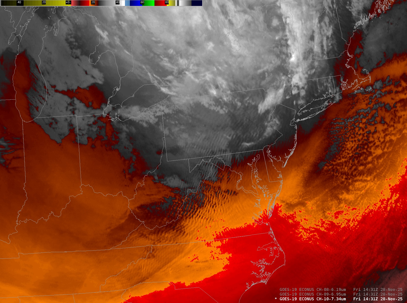
However, what if there’s not enough moisture for condensation to happen? Can these waves still be seen? If you’re looking using a water vapor channel, then the answer is yes. Look at the following animation of the 7.34 micron (low level water vapor) band from GOES-19. Note now in eastern Virginia and North Carolina, even though skies are clear the same wave pattern is visible. There’s even a particularly interesting feature in central Virginia where eastward-moving flow is creating its own waves that are intersecting with the westward flow over the Appalachian Mountains which is creating wave interference.
These events matter because these mountain waves are a significant cause of clear air turbulence (CAT). Turbulence associated with convection is easier for aircraft pilots and flight planners to identify and avoid since it is found in the vicinity of deep, moist convection. CAT, on the other hand, is not visible to the naked eye at standard visible wavelengths, but water vapor imagery can help pilots avoid these situations.
It’s important to note that the Channel 10 (7.34 micron) channel shown above is largely sensitive to low level water vapor. The waves depicted here are unlikely to disturb aviation too much as they are occurring at a level where most planes are just passing through on their way up to cruising altitudes or down to airports. However, these waves are still visible on the upper level water vapor channel, Channel 6 (6.19 microns).
View only this post Read Less


