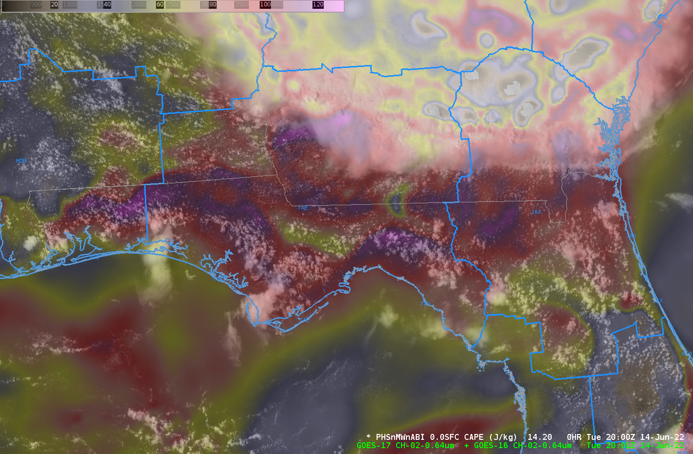
This website works best with a newer web browser such as Chrome, Firefox, Safari or Microsoft Edge. Internet Explorer is not supported by this website.

Satellite detection of ice

A colder-than-normal February over the western Great Lakes (through the 27th, Duluth is 10o F below normal; Marquette is 5o F below normal; Green Day is 2o F below normal; Cleveland is 1o F below normal) has fostered a growth in ice cover over the Lakes (This figure, from here, for... Read More

A colder-than-normal February over the western Great Lakes (through the 27th, Duluth is 10o F below normal; Marquette is 5o F below normal; Green Day is 2o F below normal; Cleveland is 1o F below normal) has fostered a growth in ice cover over the Lakes (This figure, from here, for example). How can satellites detect that ice, especially for a region where winter-time cloudiness is notorious? In general, there are two different ways to detect ice: Visible/Infrared imagery and Microwave imagery. The toggle above shows Advanced Technology Microwave Sounder (ATMS) ice detection (using MiRS algorithms and data from Suomi-NPP (1807 UTC) and NOAA-20 (1859 UTC)) over the Great Lakes on 25 February 2022. (These data come from the Direct Broadcast antenna at CIMSS, and are processed using CSPP to produce AWIPS-ready tiles that are available via an LDM feed). A big challenge with this field is the very large ATMS footprint. Note that these sea-ice concentration values are quantitative: values change based on how much ice is within the footprint but are also dependent on view angle.

VIIRS data (as shown at the VIIRS Today website, for example) can also be used to infer regions of ice in a qualitative sense, as shown below. The true color imagery shows possible ice features over the lakes. It’s a challenge, however, to use a single VIIRS image to distinguish (mostly) stationary ice from (usually) moving clouds. Multispectral VIIRS imagery means (via the use below of the 2.25 µm M11 band) ice features are cyan colored and can be qualitatively distinguished from clouds. Consider, for example, the color difference in the False Color image between the clouds over eastern Lake Superior (white in both True- and False-Color) and near-shore ice over southern and eastern Lake Superior (white in the True-Color and cyan in the False-Color). There are also VIIRS-based Ice Concentration products that can be computed in clear skies.

Suomi-NPP VIIRS True- and False-Color imagery over the Great Lakes, 1806 UTC on 25 February 2022 (Click to enlarge)

For cloudy regions, Advanced Baseline Imagery can be used to create estimates of Ice Surface Temperature and Ice Concentration. Quantitative estimates such as these give more information than the qualitative estimates shown above. These estimates at present are only created hourly; in partly-cloudy regions, that cadence is sufficient to give lake-wide quantitative estimates of ice coverage and temperature. CONUS imagery — with a 5-minute time cadence — and mesoscale sectors — with 1-minute cadences — can be used to monitor (in a qualitative sense) how ice is moving (as shown link, for example). High temporal-resolution imagery is important because ice sheets can change rapidly under strong winds, as shown in this tweet. At high latitudes, there are also ways of monitoring ice motion via polar orbiters (link).

GOES-16 Estimates of Ice Surface Temperatures, 1800 and 1900 UTC on 25 February 2022 (Click to enlarge)
GOES-16 Estimates of Ice Concentration, 1800 and 1900 UTC on 25 February 2022 (Click to enlarge)

A much higher-resolution method of viewing ice (again, in a qualitative, not quantitative sense) in regions of both clear and cloudy skies, day or night, is through the use of Synthetic Aperture Radar (SAR). Data are available for each Great Lake at this link. Imagery for each Lake over the past days is available there, albeit infrequently (usually around 0000 and 1200 UTC only) and over small domains. This qualitative imagery, however, is very high-resolution and gives very impressive details. Imagery over Lake Erie is shown below.

RCM estimates of Lake Erie Ice, 24-27 February 2022 (Click to — greatly! — enlarge)

VIIRS and ABI give both qualitative (false-color, visible imagery) and quantitative (ice concentration and ice temperature) depictions of ice over the lakes — or over coastal waters around Alaska. Microwave data also gives quantitative estimates (ice concentrations with large microwave footprints) and qualitative estimates (SAR data). Use all products to create a clear picture of ice coverage.

View only this post Read Less

Using NUCAPS and GOES-16 Level 2 Stability products and LightningCast to anticipate lightning

LightningCast (available here) is a CIMSS-developed product (created at the request of OPC and WPC) designed to relate current ABI fields (Band 2 (0.64 µm), 5 (1.61 µm), 13 (10.3 µm) and 15 (12.3 µm)) to the likelihood of future lightning. (A short training video on this product is available... Read More

LightningCast Probability over Atlantic Ocean, 1731 – 1816 UTC on 25 February 2022, along with ABI imagery and GLM observations (Click to enlarge)

LightningCast (available here) is a CIMSS-developed product (created at the request of OPC and WPC) designed to relate current ABI fields (Band 2 (0.64 µm), 5 (1.61 µm), 13 (10.3 µm) and 15 (12.3 µm)) to the likelihood of future lightning. (A short training video on this product is available here) In the animation above, probability contours are shown (blue: 10%; cyan: 25%; green: 50%; magenta: 75%) for the 45 minutes between 1731 and 1816 UTC, overlain on a sandwich-type RGB that includes visible imagery and enhanced Band 13 imagery for cold cloud tops. Of particular interest for this blog post is the region that develops east of Delmarva (as indicated in this image at 1751 UTC); probabilities increase there starting at 1741 and the first lightning is observed by GLM at 1756 UTC and it becomes more constant by 1806 UTC.


The GOES-16 Band 13 imagery at 1701 UTC — 45 minutes before the onset of the LightningCast — and derived Lifted Index shows convection approaching a ribbon of lower stability (show in yellow) to the east of North Carolina. That stability product is suggesting: this is where convection is most likely to strengthen because stability is lower here. Then 45 minutes later, the LightningCast probability increases and lightning is observed!

GOES-16 Band 13 (10.3 µm) imagery, with derived Stability Indices (in clear air skies) at 1701 UTC on 25 February 2022 (Click to enlarge)

As noted in this blog post, some Level 2 products from GOES-R are clear sky only. The timing of this event was such that NUCAPS profiles could be used to fill in information where clouds obscure what is occurring (GOES level 2 stability product-wise). A challenge is that NUCAPS and GOES Stability products don’t match well (that is, it’s not easy to create a NUCAPS Lifted Index). The Total Totals Index derived from NUCAPS is shown below. (This figure shows the Retrieval Status of the profiles used). A corridor of instability is present where lightning-produced convection subsequently developed.

Gridded NUCAPS fields of Total Totals index at 1716 UTC on 25 February 2022 (click to enlarge)

Use GOES-R Stability indices and NUCAPS stability indices to identify regions where LightningCast might be needed in the future to highlight where lightning might occur. The synthesis of the different products is very helpful to creating the best forecast. AWIPS imagery in this blog post was created using the NOAA/NESDIS TOWR-S AWIPS Cloud Instance. Thank you!

View only this post Read Less

Industrial plumes (and an undular bore) across parts of Texas

GOES-16 (GOES-East) Day Snow-Fog RGB and Day Cloud Phase Distinction RGB images (above) showed numerous industrial plumes — likely from power plants — streaming southward over parts of Texas on 24 February 2022. Particles emitted from power plant stacks acted to “seed” the surrounding supercooled water cloud droplets, creating a higher concentration of smaller cloud droplets... Read More

GOES-16 Day Snow-Fog RGB and Day Cloud Phase Distinction RGB images [click to play animated GIF | MP4]

GOES-16 (GOES-East) Day Snow-Fog RGB and Day Cloud Phase Distinction RGB images (above) showed numerous industrial plumes — likely from power plants — streaming southward over parts of Texas on 24 February 2022. Particles emitted from power plant stacks acted to “seed” the surrounding supercooled water cloud droplets, creating a higher concentration of smaller cloud droplets — which were more efficient reflectors of incoming solar radiation, making the plumes appear brighter. Farther to the east, the tightly-spaced cloud bands of an undular bore were also apparent (1901 UTC image).

A higher-resolution view of these features was provided by a sequence of NOAA-20 VIIRS True Color RGB, False Color RGB, Visible and Near-Infrared images (below).

NOAA-20 VIIRS True Color RGB, False Color RGB, Visible and Near-Infrared images [click to enlarge]

View only this post Read Less

Combining GOES-R and NUCAPS TPW fields in AWIPS

Total Precipitable Water is a Level 2 Derived Product created from ABI (and ancillary) data (link to information on this product) The image above shows the product at 1900 UTC on 24 February 2022. It is immediately apparent that cloudy regions have no data! There are ways to fill in those gaps at different times... Read More

GOES-16 Total Precipitable Water, 1900 UTC on 24 February 2022 (Click to enlarge)

Total Precipitable Water is a Level 2 Derived Product created from ABI (and ancillary) data (link to information on this product) The image above shows the product at 1900 UTC on 24 February 2022. It is immediately apparent that cloudy regions have no data! There are ways to fill in those gaps at different times of day.

NUCAPS thermodynamic profiles in AWIPS are derived from data from the CrIS (Cross-track Infrared Sounder) and ATMS (Advanced Technology Microwave Sounder) instruments on board NOAA-20. That thermodynamic data can be used to create fields of Total Precipitable Water, as shown below. Of course, the NUCAPS swath is limited geographically to the width of the CrIS and ATMS swaths, but values are created in clear and cloudy regions. Note that in AWIPS (which display system was used to create the imagery in this blog post) the gridded NUCAPS field has a different default color enhancement than what is shown below; create an AWIPS Procedure to load and enhance the swath with the same GOES-R enhancement used as a default in the image above.

Gridded NUCAPS estimates of Total Precipitable Water, 1900 UTC on 24 February 2022 (click to enlarge)

If you combine both the GOES-R TPW estimates with NUCAPS estimates at the same time, you will get enhanced coverage in regions where interesting weather might be happening (near gradients in TPW, for example) beneath cloud cover. NOAA-20 NUCAPS swaths occur every 90 minutes in the afternoon. moving east to west across the CONUS. Thus, at 1730 UTC, a NUCAPS TPW swath was available over the eastern part of the United States, and it could be combined with GOES-R values at that time, as shown at bottom. At 2030 UTC, a swath along the west coast (not showed) occurred. A similar set of swaths will occur east-to-west between about 0530 UTC and 1000 UTC in the morning.

GOES-16 and NUCAPS Total Precipitable Water, 1900 UTC 24 February 2022 (click to enlarge)
GOES-16 and NUCAPS Total Precipitable Water, 1730 UTC 24 February 2022 (click to enlarge)

AWIPS users can create a procedure to load gridded TPW fields in conjunction with GOES-R TPW fields, and use them as needed. AWIPS imagery in this blog post was created using the NOAA/NESDIS TOWR-S AWIPS Cloud Instance.

View only this post Read Less