

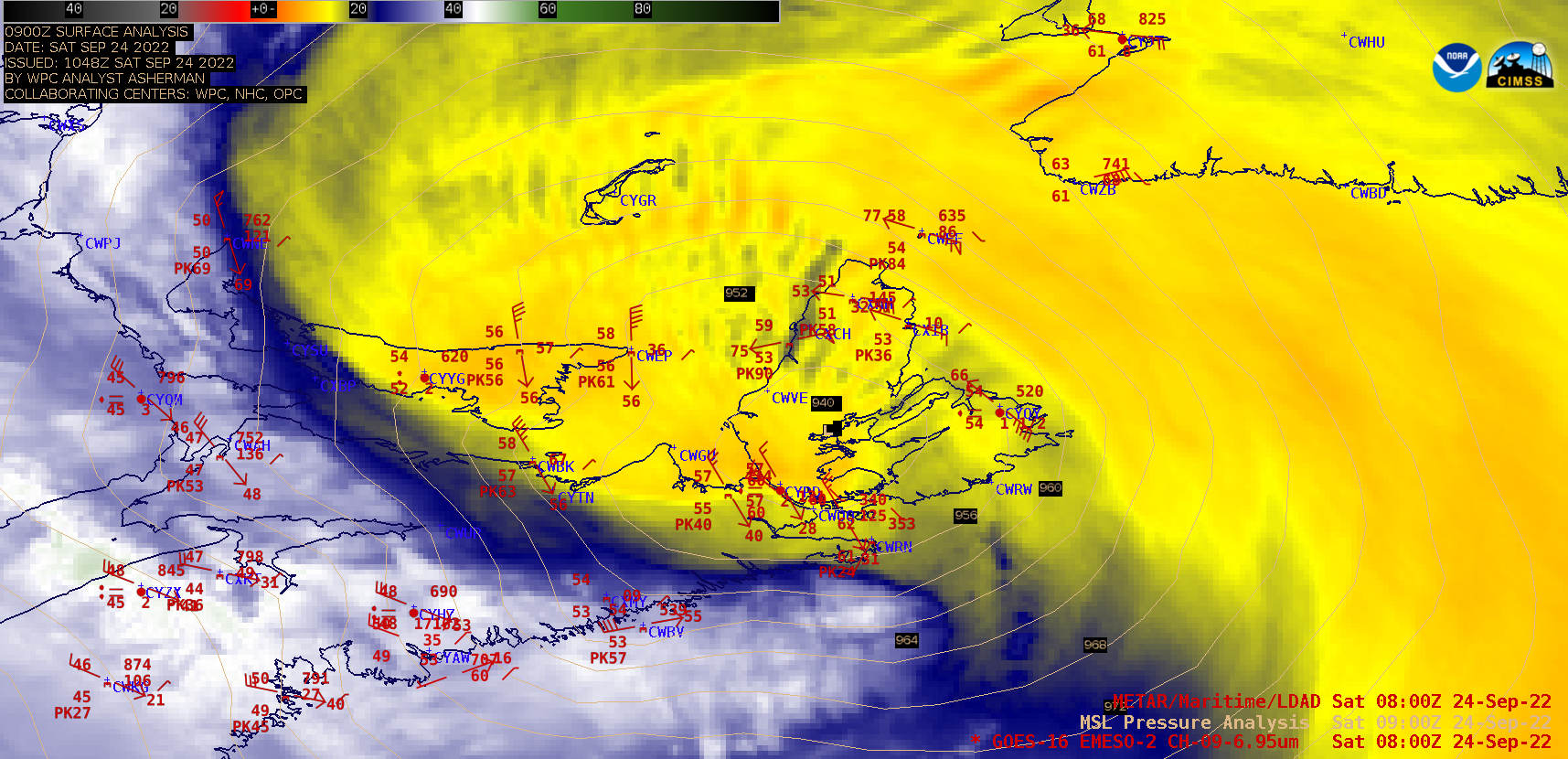
GOES-16 Mid-level Water Vapor (6.9 µm) images [click to play animated GIF | MP4]
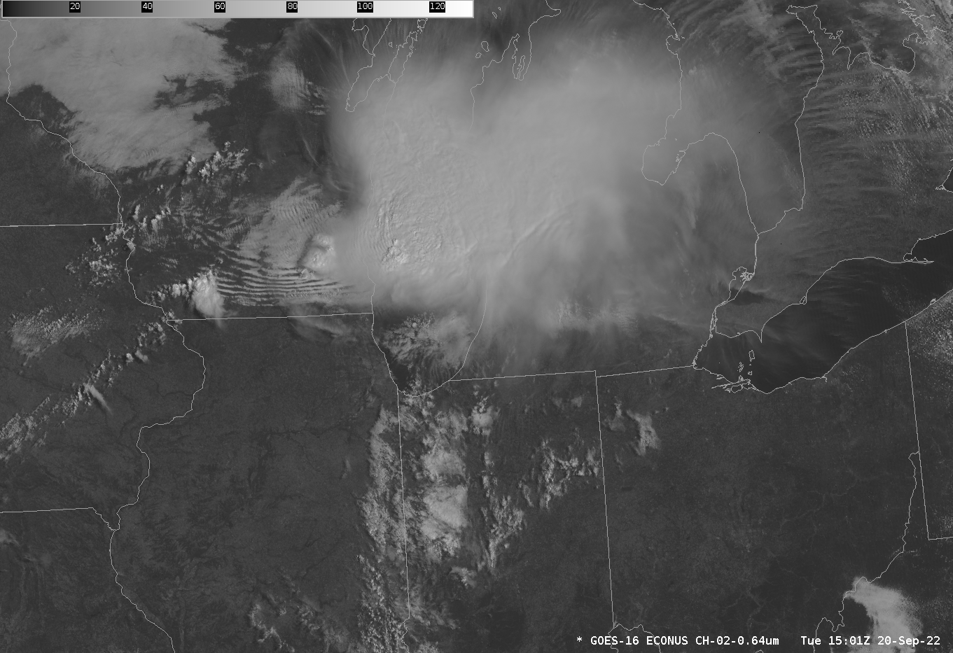
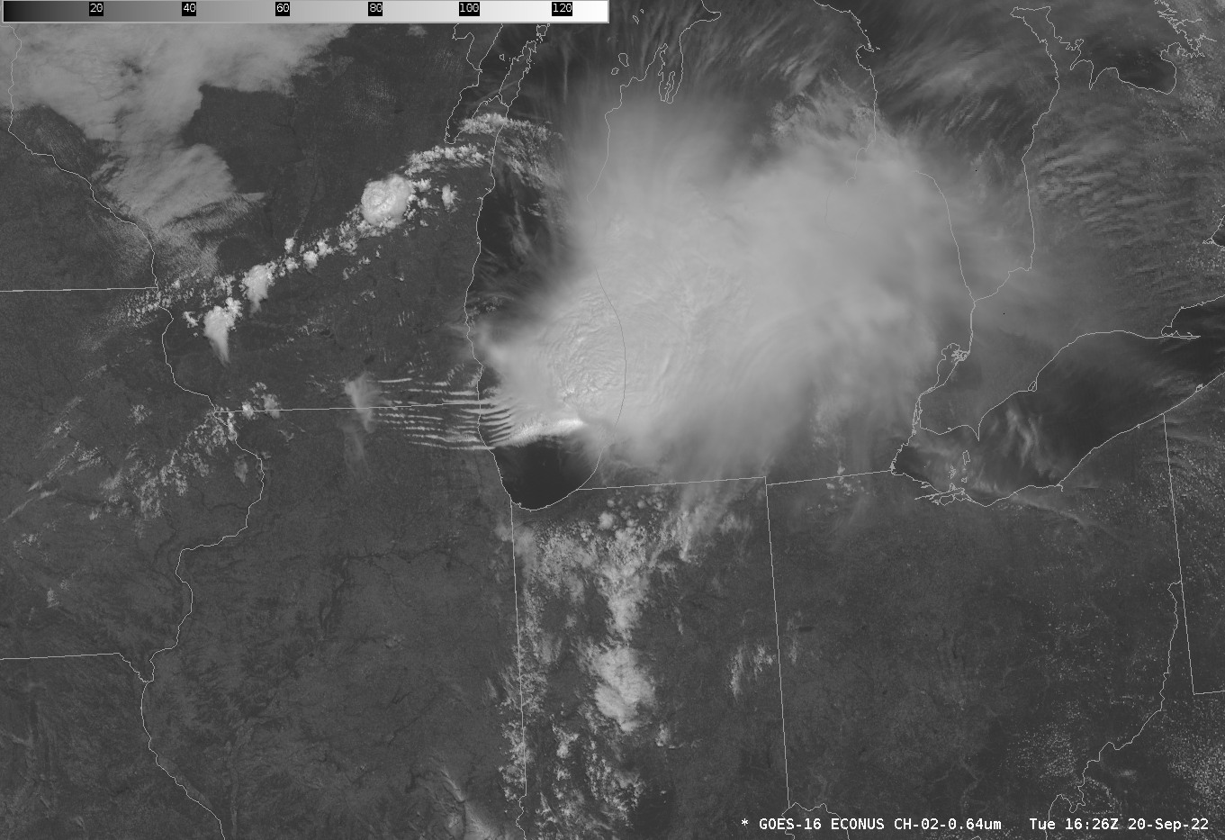
One feature of interest was a region of lee waves generated by strong easterly boundary layer winds interacting with the Highlands terrain in the northern portion of Cape Breton Island — these waves spread westward across parts of the Gulf of Saint Lawrence (below).
Comparison of GOES-16 Water Vapor image at 0700 UTC and topography [click to enlarge]
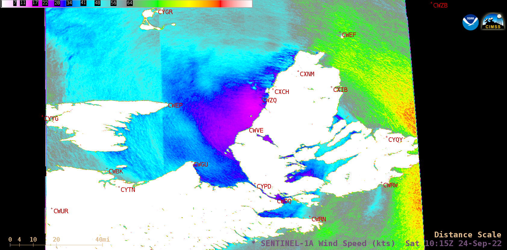
Sentinel-1A Synthetic Aperture Radar (SAR) winds at 1015 UTC [click to enlarge]
The animation of GOES-16 airmass RGB, below, shows the evolution of Fiona and its interaction with a Potential Vorticity Maximum (orange/red in the RGB).
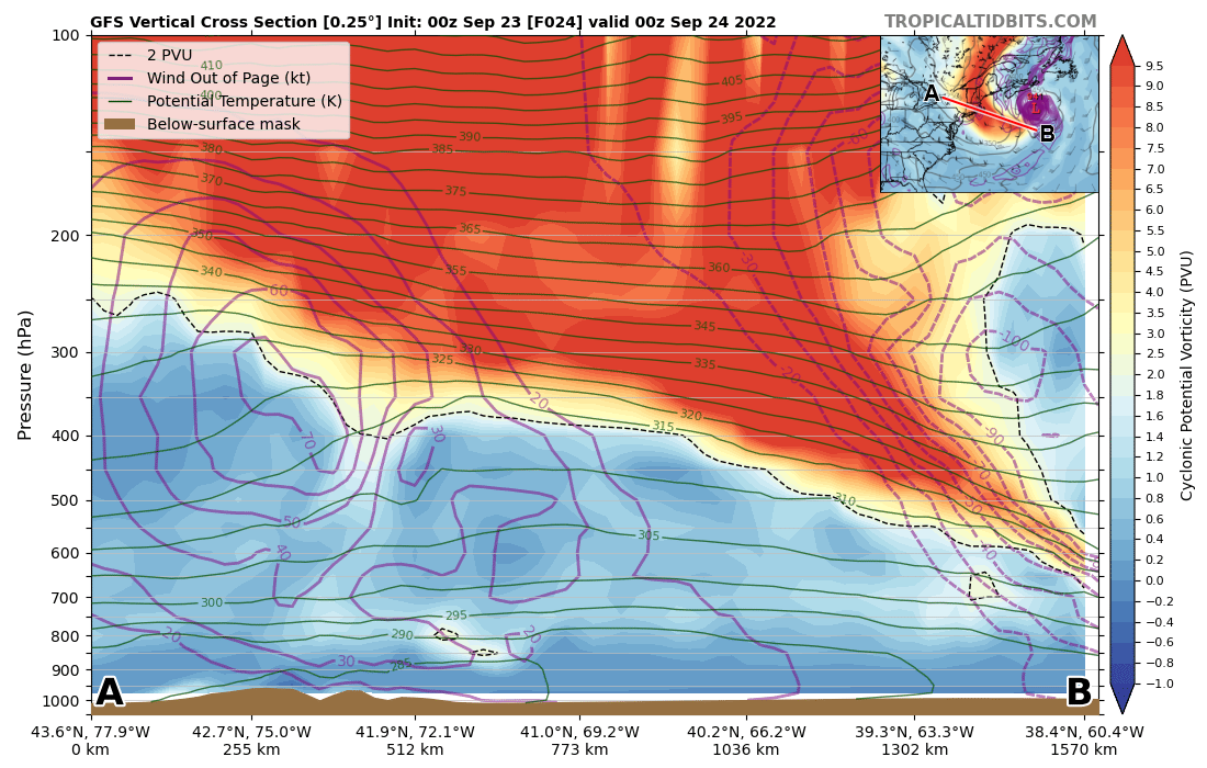
Perhaps you are skeptical that the Orange/Red signature in the Airmass RGB is a Potential Vorticity Signature. Consider the animation below, downloaded from the TropicalTidbits website and showing 00 – 30 hour GFS model output from the run initialized at 0000 UTC on 23 September. A rich source of cyclonic potential vorticity air (in orange) wraps around Fiona as it moves north. Similar behavior is apparent in the Airmass RGB animation above. This cross section (also from the excellent Tropical Tidbits site) of the model data (24 h into the forecast run) also shows a classic stratospheric intrusion structure.
This collection of training videos from ECCC includes one from Chris Fogarty (scroll down at that website) that includes an in-depth post-storm analyses of the landfall.
View only this post Read Less


