
GOES-17 (GOES-West) “Red” Visible (0.64 µm), Shortwave Infrared (3.9 µm), “Clean” Infrared Window (10.35 µm) and Fire Temperature RGB images (above) showed a wildfire just southeast of Fort Simpson in Canada’s Northwest Territories (just north of the border with British Columbia), which produced a pair of pyrocumulonimbus (pyroCb) clouds late in the day on 10 October 2022. Surface winds gusting... Read More
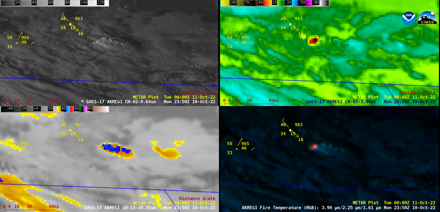
GOES-17 “Red” Visible (0.64 µm, top left), Shortwave Infrared (3.9 µm, top right), “Clean” Infrared Window (10.3 µm, bottom left) and Fire Temperature RGB (bottom right) images [click to play animated GIF | MP4]
GOES-17
(GOES-West) “Red” Visible (
0.64 µm), Shortwave Infrared (
3.9 µm), “Clean” Infrared Window (
10.35 µm) and
Fire Temperature RGB images
(above) showed a wildfire just southeast of
Fort Simpson in Canada’s Northwest Territories (just north of the border with British Columbia), which produced a pair of
pyrocumulonimbus (pyroCb) clouds late in the day on 10 October 2022. Surface winds gusting as high as 28 knots (32 mph) at Fort Simpson — in the wake of a cold frontal passage (
surface analyses) — likely played a role in helping to intensify the fire enough to produce the 2 pyroCb clouds. The hottest 3.9 µm infrared brightness temperature sampled in the 10-minute imagery was 121.19ºC at 2000 UTC — with the pyroCb clouds developing around 2200 and 2330 UTC.
A toggle between Suomi-NPP VIIRS Visible (0.64 µm) images at 1903 and 2042 UTC (below) displayed the large smoke plume that drifted southeastward as far as northern Saskatchewan. About 200 miles southeast of the wildfire source region, this smoke reduced the surface visibility to 3 miles or less at Hay River NT around 21 UTC.
Suomi-NPP VIIRS Visible (0.64 µm) images at 1903 and 2042 UTC [click to enlarge]
During the subsequent nighttime hours, a toggle between Suomi-NPP VIIRS Shortwave Infrared (3.74 µm) and Day/Night Band (0.7 µm) images at 1211 UTC
(below) revealed the thermal signatures and visible glow of individual active fires around the periphery of the fire complex.
Suomi-NPP VIIRS Shortwave Infrared (3.74 µm) and Day/Night Band (0.7 µm) images at 1211 UTC [click to enlarge]
GOES-17 and GOES-16
(GOES-East) True Color RGB images from the
CSPP GeoSphere site
(below) showed the hazy smoke plume as it drifted southeastward — along with the pyrocumulus and pyroCb clouds that developed over the wind-driven fire complex.
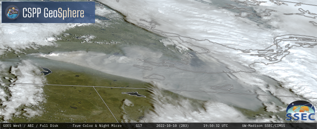
GOES-17 True Color RGB images [click to play MP4 animation]
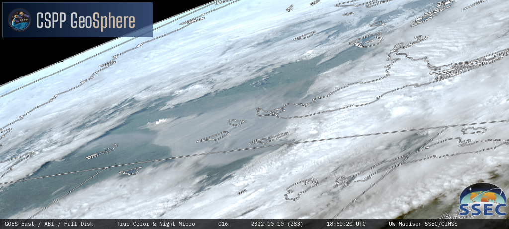
GOES-16 True Color RGB images [click to play MP4 animation]
View only this post
Read Less


