This website works best with a newer web browser such as Chrome, Firefox, Safari or Microsoft
Edge. Internet Explorer is not supported by this website.
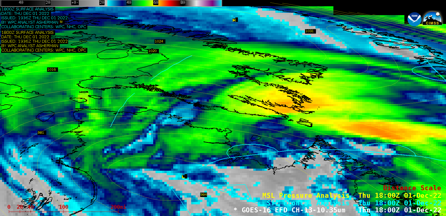
After 1800 UTC on 01 December 2022, changes were made to Full Disk GOES-16 (GOES-East) imagery that is distributed via the Satellite Broadcast Network (SBN) for AWIPS users (see the bottom section of this TOWR-S Communications). One change was the increase in spatial resolution of the ABI Band 13 “Clean” Infrared... Read More
GOES-16 “Clean” Infrared Window (10.3 µm) images [click to play animated GIF | MP4]
After 1800 UTC on 01 December 2022, changes were made to Full Disk GOES-16 (GOES-East) imagery that is distributed via the Satellite Broadcast Network (SBN) for AWIPS users (see the bottom section of this TOWR-S Communications). One change was the increase in spatial resolution of the ABI Band 13 “Clean” Infrared Window (10.3 µm) data from 6 km to the native 2 km (at satellite nadir) — as shown in an animation of imagery in the vicinity of a low pressure system located over northern Quebec, Canada (above). A toggle between those “before” (1800 UTC) and “after” (1810 UTC) images is available here.
GOES-16 Infrared imagery in the tropics (below) displayed convection along the Intertropical Convergence Zone (ITCZ) in the East Pacific Ocean. A toggle between those “before” and “after” images is available here.
GOES-16 “Clean” Infrared Window (10.3 µm) images [click to play animated GIF | MP4]
Another GOES-16 Infrared example centered over southern British Columbia, Canada is shown below. A toggle between those “before” and “after” images is available here.
GOES-16 “Clean” Infrared Window (10.3 µm) images (credit: Tim Schmit, NOAA/NESDIS/ASPB) [click to enlarge]
One other important change is that “Full Disk” imagery will only cover the Northern Hemisphere, as shown in an animation of GOES-16 Mid-level Water Vapor (6.9 µm) images (below).
GOES-16 Mid-level Water Vapor (6.9 µm) images [click to play animated GIF | MP4]
One of the gases emitted from the Mauna Loa eruption is SO2. The 0223 UTC 30 November update from this site notes that emission rates of approximately 250,000 tonnes [sic] per day were measured on 28 November! What satellite products can be used to diagnose this gas qualitatively and quantitatively? There is... Read More
SO2 (top) and Ash (bottom) RGBs over Mauna Loa, 2026 UTC on 29 November through 1156 UTC on 30 November 2022 (Click to enlarge)
One of the gases emitted from the Mauna Loa eruption is SO2. The 0223 UTC 30 November update from this site notes that emission rates of approximately 250,000 tonnes [sic] per day were measured on 28 November! What satellite products can be used to diagnose this gas qualitatively and quantitatively? There is an SO2 RGB created with GOES-R channels, so GOES-17 and GOES-18 are available to monitor SO2 qualitatively. The animation above shows both the SO2 and Ash RGBs over Hawaii, at half-hourly intervals. The light green regions around and downstream of Mauna Loa highlight parts of the lower troposphere that are rich in SO2. (Here is the SO2 RGB Quick Guide).
Longer animations using 5-minute images of GOES-17 Ash RGB and SO2 RGB imagery — from 1801 UTC on 29 November to 1501 UTC on 30 November — are shown below.
GOES-17 Ash RGB and SO2 RGB images, from 1801 UTC on 29 November to 1501 UTC on 30 November (credit: Scott Bachmeier, CIMSS) [click to play animated GIF | MP4]
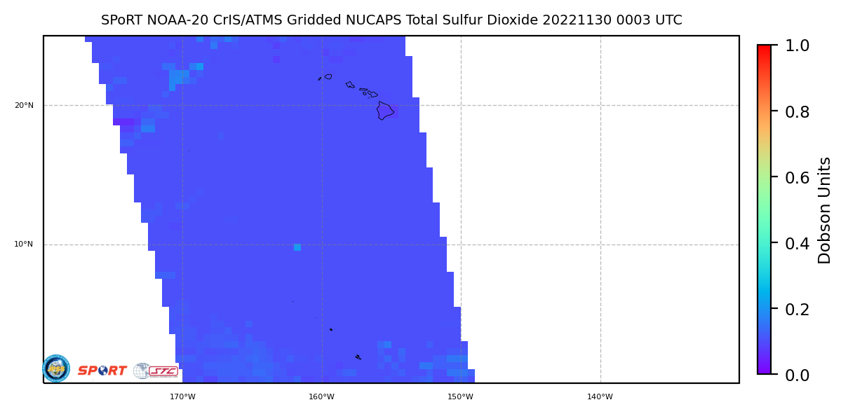
Total Sulfur Dioxide as measured by NOAA-20 NUCAPS Profiles, 0003 UTC on 30 November 2022 (Click to enlarge)
Gridded NUCAPS fields available at this site from SPoRT include SO2 concentrations, as shown above. A minor increase in SO2 concentration is indicated. However, the Quality indicators suggest that the NUCAPS retrievals over part of Hawai’i failed.
NASA has a global SO2 monitoring site here that shows daily qualitative imagery from OMI (on board Aura), OMPS (on board Suomi-NPP) and Tropomi. OMI imagery is here, OMPS imagery is here, and TROPOMI imagery is here. (Note that the TROPOMI imagery is not processed as quickly as OMI and OMPS imagery). The OMPS images for 28 and 29 November, shown below, show values off the scale.
SO2 concentrations as measured by the OMPS instrument on Suomi NPP, 28 and 29 November 2022 (Click to enlarge)
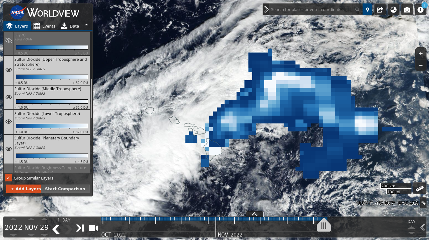
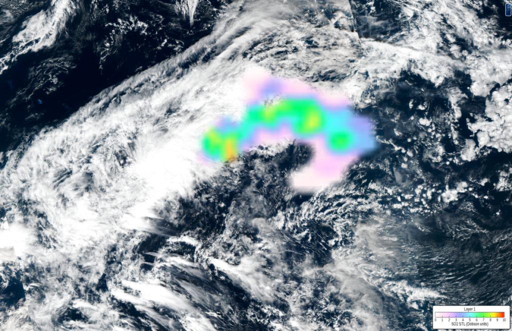
SO2 concentrations/distributions from OMI on Aura and OMPS on Suomi NPP are also available at NASA Worldview as shown below. OMPS imagery is available more quickly at NASA Worldview.
NASA Worldview image of Suomi NPP True-Color from VIIRS and SO2 concentration from OMPS, 29 November 2022 (click to enlarge)
The toggle below compares OMI (Aura) and OMPS (NPP) estimates of SO2 concentration on 28 November. Aura and NPP have similar orbits so there is little time difference between the two observations. Both show values greater than 32 DU.
OMI and OMPS estimates of SO2 concentration on 28 November 2022 (Click to enlarge)
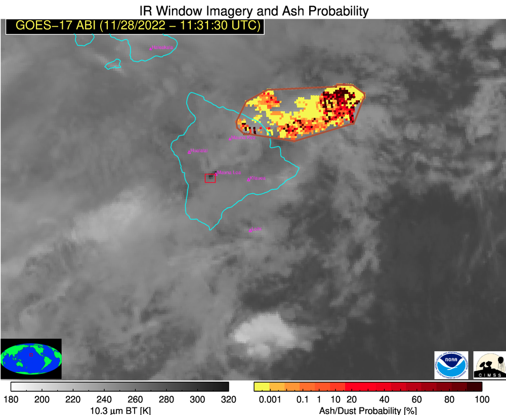
Mauna Loa on the Big Island of Hawai’i became active overnight, ending a quiescent phase that started back in 1984 — the longest period of dormancy for this Volcano since the 1800s. The Ash Probability animation above, combining both GOES-17 PACUS and GOES-17 Full Disk imagery (using imagery from this site)... Read More
GOES-17 Clean Window Infrared (10.3 µm) imagery and quantitative estimates of Ash/Dust Probability, 0906 – 1301 UTC on 28 November 2022 (Click to enlarge)
Mauna Loa on the Big Island of Hawai’i became active overnight, ending a quiescent phase that started back in 1984 — the longest period of dormancy for this Volcano since the 1800s. The Ash Probability animation above, combining both GOES-17 PACUS and GOES-17 Full Disk imagery (using imagery from this site) shows the Ash Cloud from this eruption moving northeastward from Hawai’i into the Pacific Ocean. The hot spot of the caldera is also apparent in the imagery.
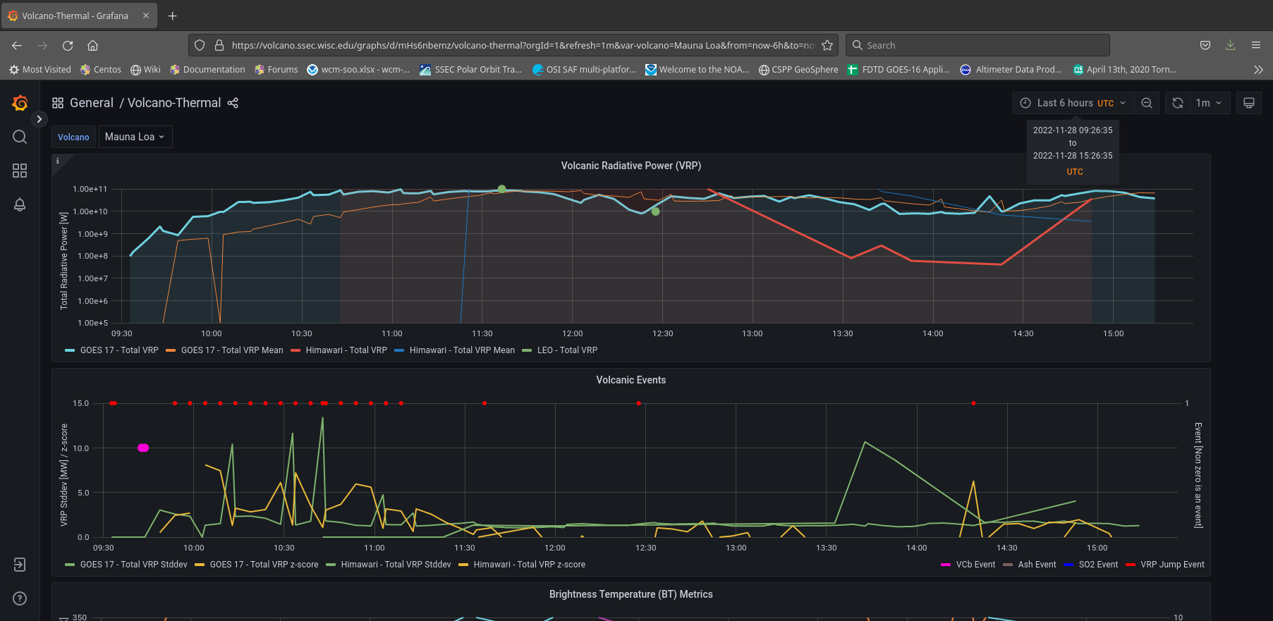
The SSEC/CIMSS Volcano Monitoring website also includes a Thermal Monitoring tab, and the information for Mauna Loa (link) from 0926 to 1526 UTC on 28 November is shown below.
Satellite Thermal Monitoring information from the SSEC/CIMSS Volcano website (https://volcano.ssec.wisc.edu), 0926 – 1526 UTC on 28 November 2022 (Click to enlarge)
Tim Schmit (NOAA STAR/ASPB) created the 16-panel animations below, one showing all GOES-17 channels and one showing all GOES-18 channels. The heat signature is very apparent at 3.9 µm — but there is also a significant contributions at 1.6 µm and 2.2 µm! The window channels (Bands 11, 13, 14 and 15 at 8.4 µm, 10.3 µm, 11.2 µm and 12.3 µm) also show the heat signature. The effects of the Loop Heat Pipe malfunction on GOES-17 are also apparent in the Band 12 and Band 16 imagery (9.6 µm and 13.3 µm) by the end of the animation; GOES-18 has a more pristine look. Post-launch check-outs for GOES-18 continue, and it is scheduled to become operational as GOES-West in January of 2023. (GOES-18 data in the animation are preliminary and non-operational).
16-Panel showing all GOES-17 bands over Hawai’i, 0911 – 1206 UTC on 28 November 202216-Panel showing all GOES-18 bands over Hawai’i, 0916 – 1211 UTC on 28 November 2022
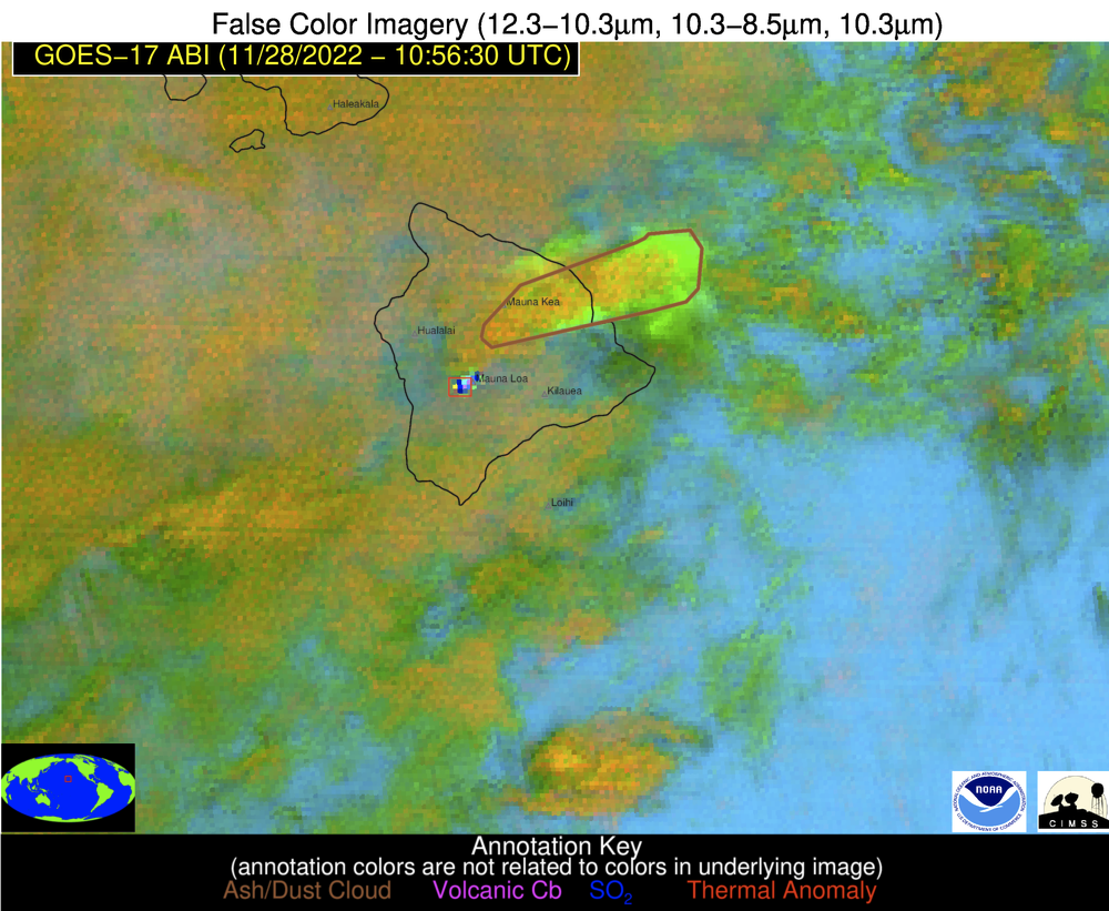
The animation below shows the Clean Window Infrared (10.3 µm) and the Fire Temperature RGB. Note the ash cloud in the 10.3 µm imagery is difficult to distinguish from other clouds, except by inferring a connection to the sudden hot spot in the Fire Temperature RGB. Channel difference products, however, such as the Split Cloud Top Phase (11.2 µm – 8.4 µm), shown underneath the animation below, do highlight the ash cloud (compare the signals in the Ash Cloud stretching east-northeast of Hawai’i with the cloud approaching Hawai’i from the southwest), as would RGBs that incorporate that difference field (that is, the Ash RGB, a variation of which is available at the SSEC/CIMSS volcano website, from both ABI and VIIRS data).
GOES-17 Band 13 (Clean Window) Infrared (10.3 µm) with the Fire Temperature RGB (combining 3.9 µm, 2.2 µm and 1.6 µm), 0916 – 1401 UTC on 28 November 2022 (Click to enlarge)GOES-17 Clean Window (10.3 µm) and GOES-17 Split Cloud Phase Difference (11.2 µm – 8.4 µm) at 1056 UTC on 28 November 2022, both on top of the Fire Temperature RGB (Click to enlarge)
Larger-scale animations of GOES-17 Ash RGB and SO2 RGB images (below) exhibited a strong signature of SO2 within the volcanic cloud — particularly the segment that drifted east-northeastward away from the Big Island of Hawai`i during the 0931-2101 UTC period.
GOES-17 Ash RGB and SO2 RGB images (credit: Scott Bachmeier, CIMSS) [click to play animated GIF | MP4]
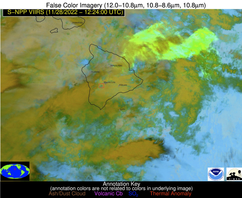
NOAA-20 overflew Hawai’i shortly after 1130 UTC, and the higher-resolution (compared to ABI) VIIRS instrument gave a good view of the eruption. The I04 (3.74 µm) channel showed such warm temperatures that wrap-around effect occurred in the imagery (the white region that is within the orange/red center of the signal), and the visible signal was so bright that a hysteresis effect is apparent downscan of the volcano in the Day Night band imagery. Note in the Day Night Band image that a very small signal is apparent over Kilauea to the southeast of Mauna Loa.
NOAA-20 VIIRS I04 (3.74 µm) and Day Night Band visible (0.70 µm) imagery 1134 UTC on 28 November 2022 (Click to enlarge); Imagery created by W. Straka III, CIMSS
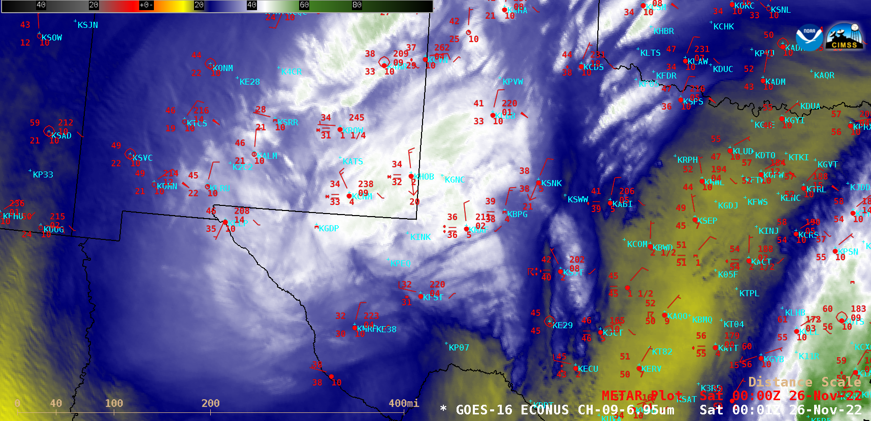
GOES-16 (GOES-East) Mid-level Water Vapor (6.9 µm) images (above) showed the circulation associated with an anomalously-deep middle tropospheric cutoff low as it moved from northern Mexico across Texas during the 1301 UTC on 25 November to 2101 UTC on 26 November 2022 time period. Elevated convective elements rotating within the cutoff low helped to... Read More
GOES-16 Mid-level Water Vapor (6.9 µm) images [click to play MP4 animation | Animated GIF]
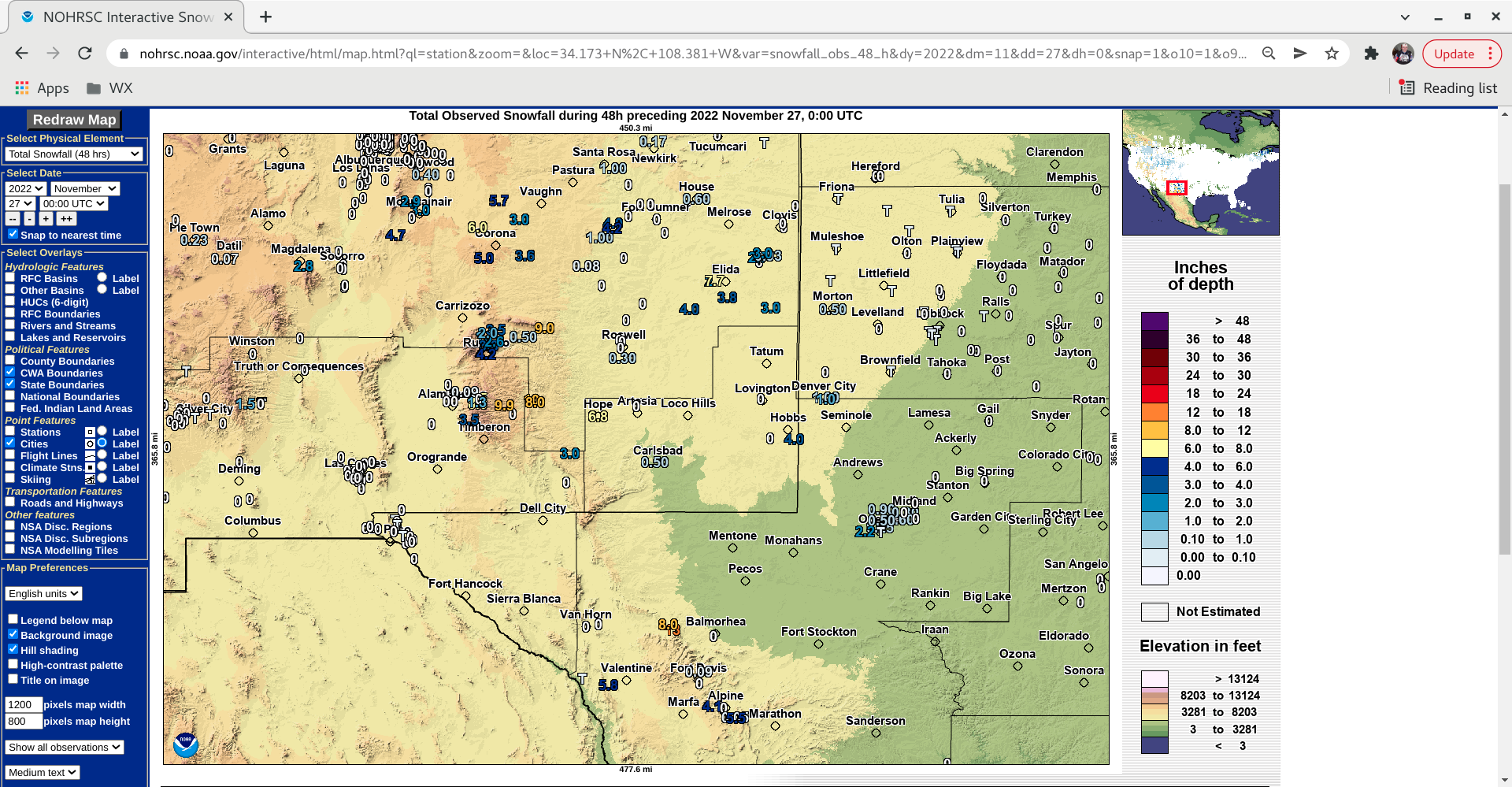
GOES-16 (GOES-East) Mid-level Water Vapor (6.9 µm) images (above) showed the circulation associated with an anomalously-deep middle tropospheric cutoff low as it moved from northern Mexico across Texas during the 1301 UTC on 25 November to 2101 UTC on 26 November 2022 time period. Elevated convective elements rotating within the cutoff low helped to enhance precipitation rates in portions of western Texas and eastern New Mexico — with accumulating snowfall occurring at many locations.
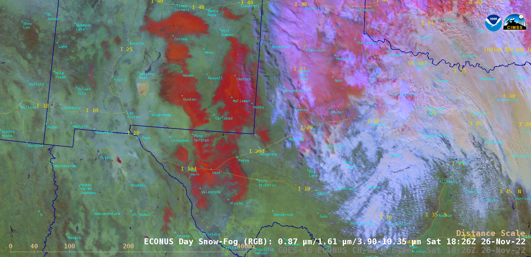
As the system moved off to the east during the day on 26 November, GOES-16 “Red” Visible (0.64 µm) and Day Snow-Fog RGB images (below) revealed the extent of snow cover (darker shades of red in the RGB imagery) across parts of southeastern New Mexico and southwestern Texas.
GOES-16 “Red” Visible (0.64 µm) and Day Snow-Fog RGB images [click to play MP4 animation | Animated GIF ]
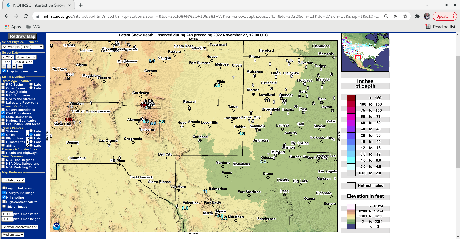
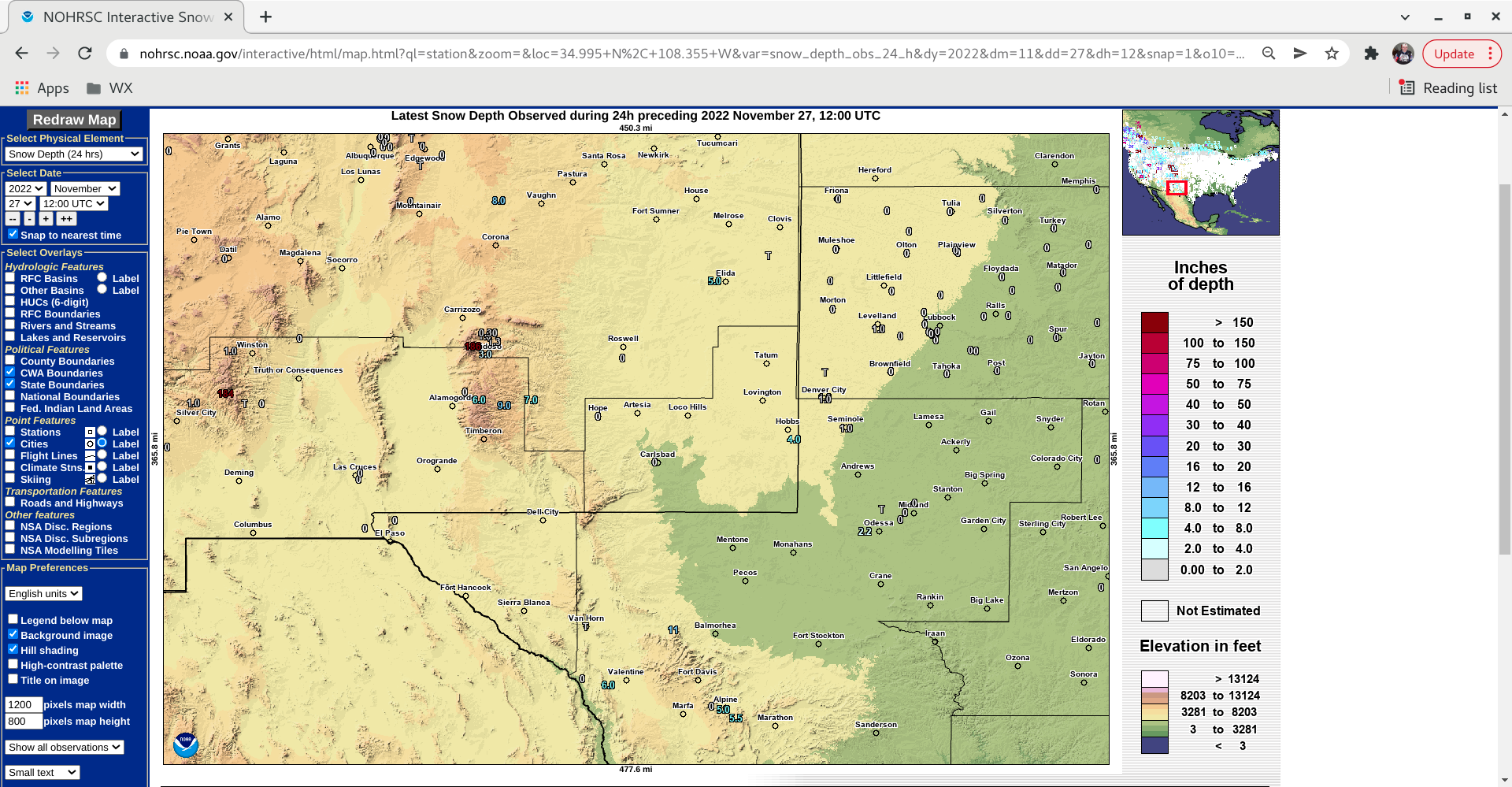
In a toggle between GOES-16 Day Snow-Fog RGB and Land Surface Temperature (LST) derived product images at 2101 UTC (below), LST values over the deepest snow cover just west of the New Mexico / Texas border were as cold as the mid 30s F (compared to 50s and 60s F over bare ground just to the east and west of that snow cover). 12 UTC snow depth reports within that patch of snow cover were 4-5 inches.
GOES-16 Day Snow-Fog RGB image and Land Surface Temperature derived product at 2101 UTC [click to enlarge]


