GOES-18 (GOES-West) SO2 RGB and Ash RGB images (above) showed the northeastward drift of a volcanic cloud produced by an eruption of Mount Shishaldin that began shortly before 0730 UTC on 23 July 2023. The initial (higher-altitude) portion of the volcanic cloud likely contained moderate concentrations of SO2 (denoted by brighter shades of yellow in the SO2 RGB images)... Read More

GOES-18 SO2 RGB and Ash RGB images, 0700-1900 UTC [click to play animated GIF | MP4]
GOES-18
(GOES-West) SO2 RGB and
Ash RGB images
(above) showed the northeastward drift of a volcanic cloud produced by an eruption of
Mount Shishaldin that began shortly before 0730 UTC on 23 July 2023. The initial (higher-altitude) portion of the volcanic cloud likely contained moderate concentrations of SO2 (denoted by brighter shades of yellow in the SO2 RGB images) — while the trailing (lower-altitude) portion of the volcanic cloud likely contained concentrations of ash (shades of pink in the Ash RGB images). The ash signature dissipated after about 4 hours, while the SO2 signature persisted for the duration of the 11.5-hour animation.
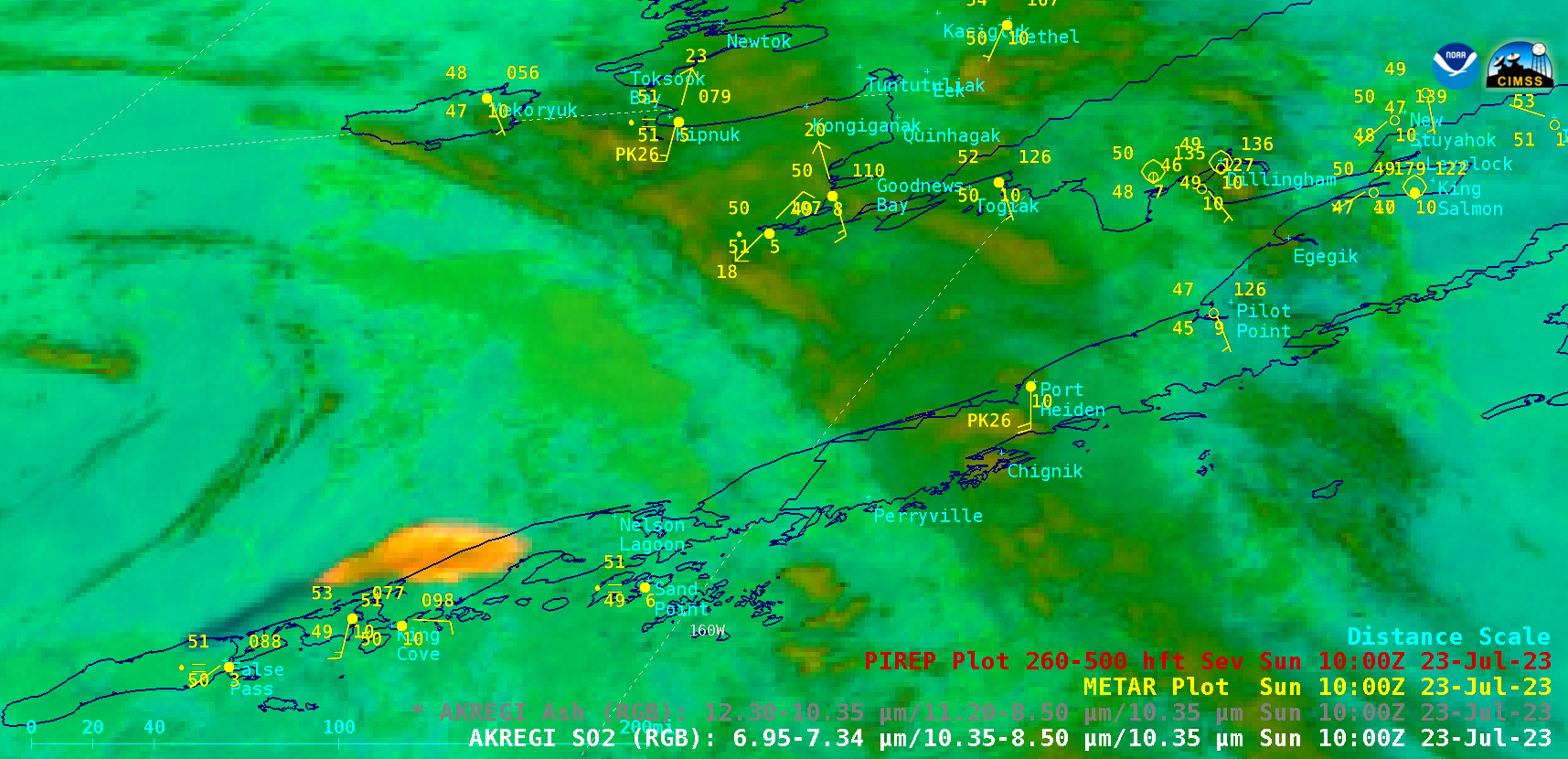
A toggle between the SO2 RGB and Ash RGB images at 1000 UTC is shown below.
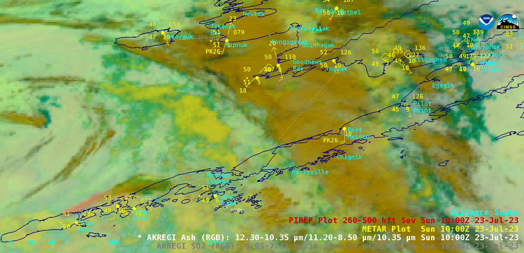
GOES-18 Ash RGB and SO2 RGB images at 1000 UTC [click to enlarge]
A pilot report issued at 0727 UTC
(below) indicated that volcanic ash (VA) was rising to altitudes of 30000 feet (FL300).
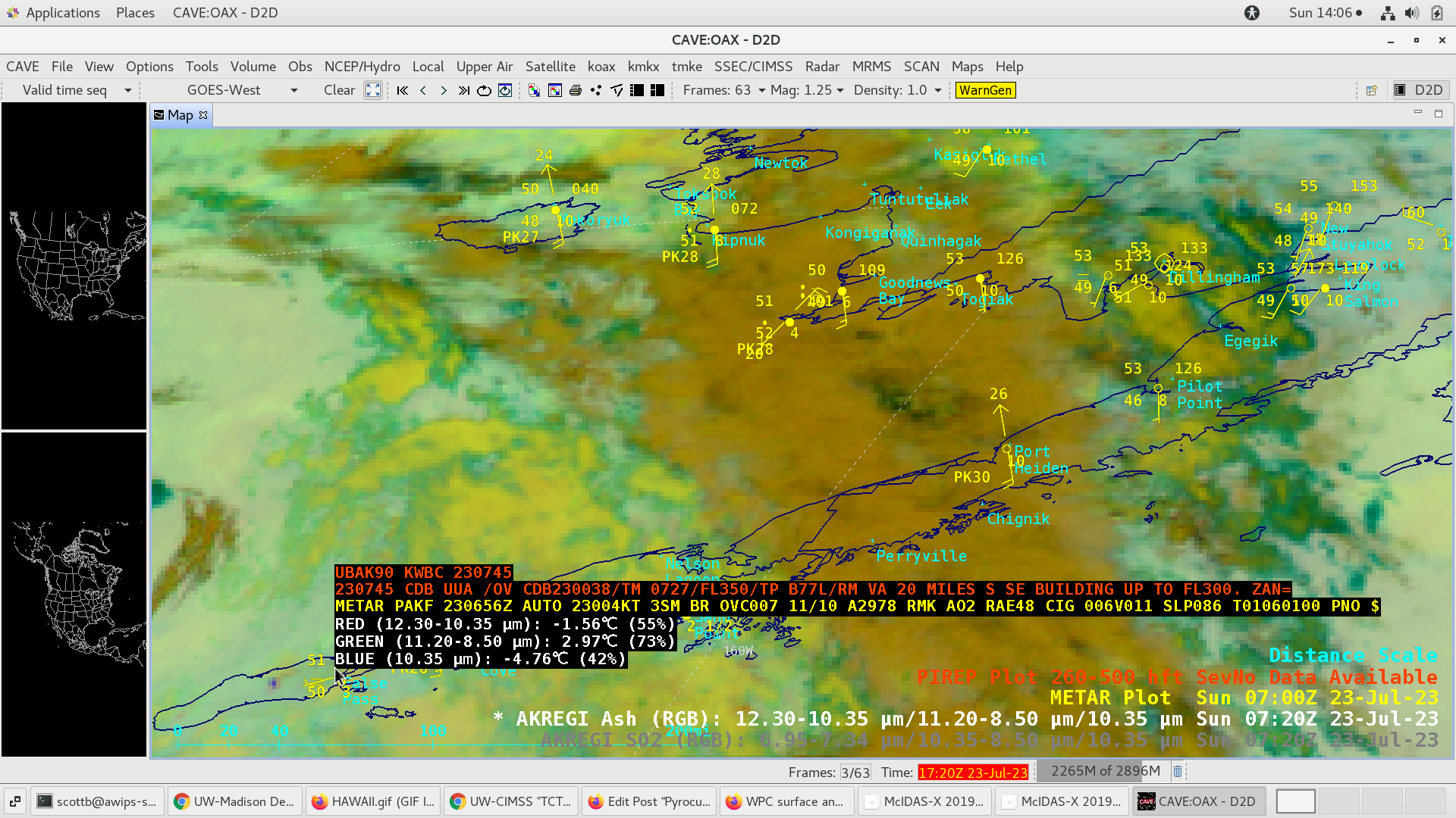
GOES-18 Ash RGB image at 0720 UTC, with cursor sampling of a Pilot Report issued at 0727 UTC [click to enlarge]
===== 24 July Update =====
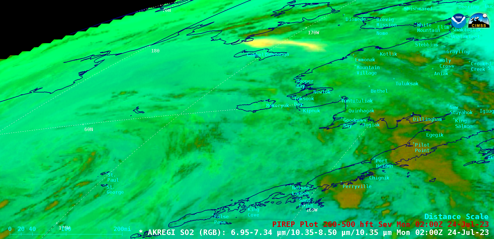
GOES-18 SO2 RGB images, 0700 UTC on 23 July to 1700 UTC on 24 July [click to play animated GIF | MP4]
A longer animation of GOES-18 SO2 RGB images
(above) showed the distinct SO2 signature (brighter shades of yellow) from the Shishaldin eruption, as it rotated counterclockwise within the circulation of a slow-moving middle tropospheric low in the Bering Sea — moving over far southwest Alaska and St. Lawrence Island on 23 July, and eventually becoming stretched into a long/narrow filament over far eastern Russia on 24 July.
View only this post
Read Less


