This website works best with a newer web browser such as Chrome, Firefox, Safari or Microsoft
Edge. Internet Explorer is not supported by this website.
10-minute Full Disk scan GOES-18 Air Mass RGB images (above) showed a cyclone as it intensified to a Hurricane Force Low by 0000 UTC on 24 December 2023 as it moved north across the Gulf of Alaska (suface analyses). Brighter orange-red hues in the RGB images highlighted a Potential Vortcity (PV) Anomaly within... Read More
GOES-18 Air Mass RGB images, with/without contours of AK-NAM40 model PV 1.5 Pressure, from 0000 UTC on 23 December to 0300 UTC on 24 December [click to play animated GIF | MP4]
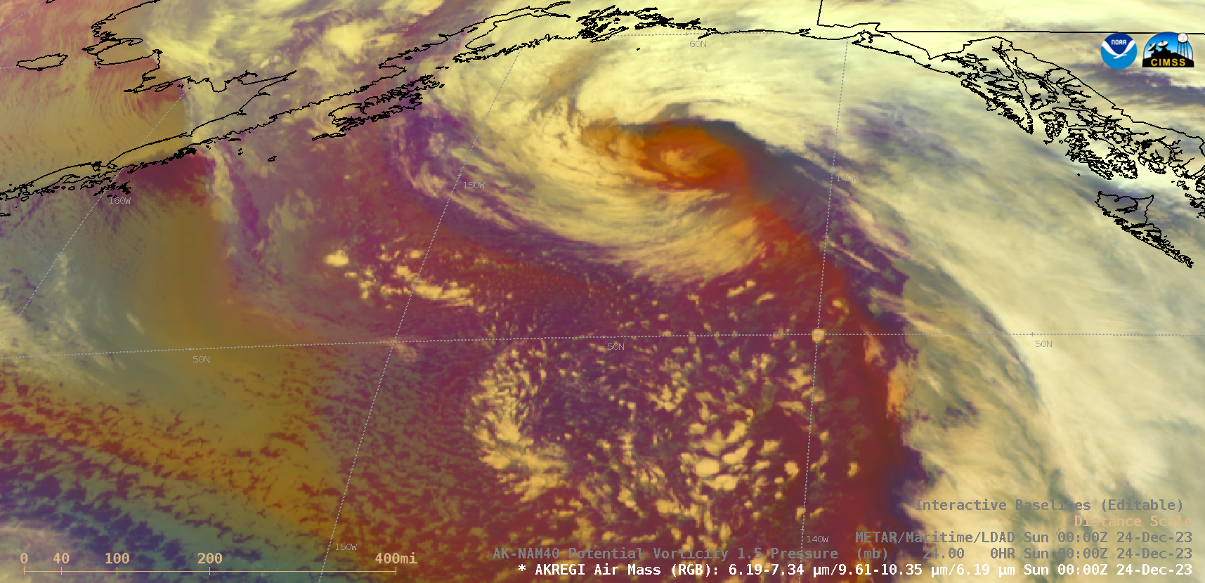
10-minute Full Disk scan GOES-18 Air Mass RGB images (above) showed a cyclone as it intensified to a Hurricane Force Low by 0000 UTC on 24 December 2023 as it moved north across the Gulf of Alaska (suface analyses). Brighter orange-red hues in the RGB images highlighted a Potential Vortcity (PV) Anomaly within the core of the low pressure system — AK-NAM40 model fields indicated that the “dynamic tropopause” (taken to be the pressure of the PV 1.5 surface) had descended to near the 800 hPa pressure level at 0000 UTC on 24 December (below).
GOES-18 Air Mass RGB image at 0000 UTC on 24 December, with/without contours of AK-NAM40 model PV 1.5 Pressure [click to enlarge]
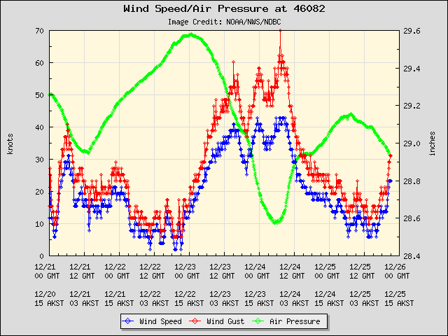
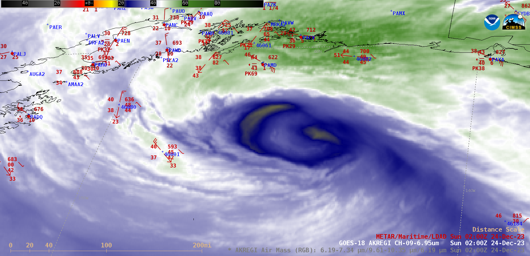
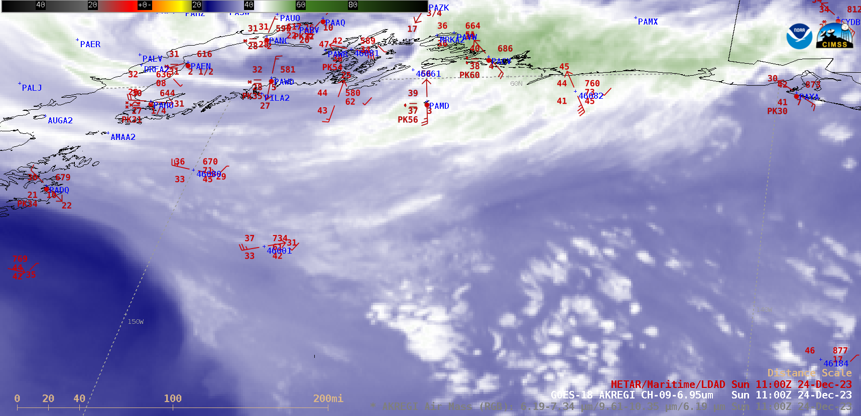
A closer view of GOES-18 Air Mass RGB and Mid-level Water Vapor (6.9 µm) images (below) displayed the low as it eventually moved inland across Southcentral Alaska by 1200 UTC on 24 December. Notable peak wind gusts included 70 knots at Buoy 46082 at 0710 UTC, 69 knots at Middleton Island (PAMD) around 0200 UTC and 60 knots at Codova (PACV) around 1100 UTC.
GOES-18 Air Mass RGB and Mid-level Water Vapor (6.9 µm) images, with plots of Surface/Buoy/Ship Reports, from 0000 UTC to 1200 UTC on 24 December [click to play animated GIF | MP4]
This Hurricane Force Low was rather anomalous in terms of its low Mean Sea Level Pressure (MSLP) and strong 925 hPa wind speeds (source), as shown below.
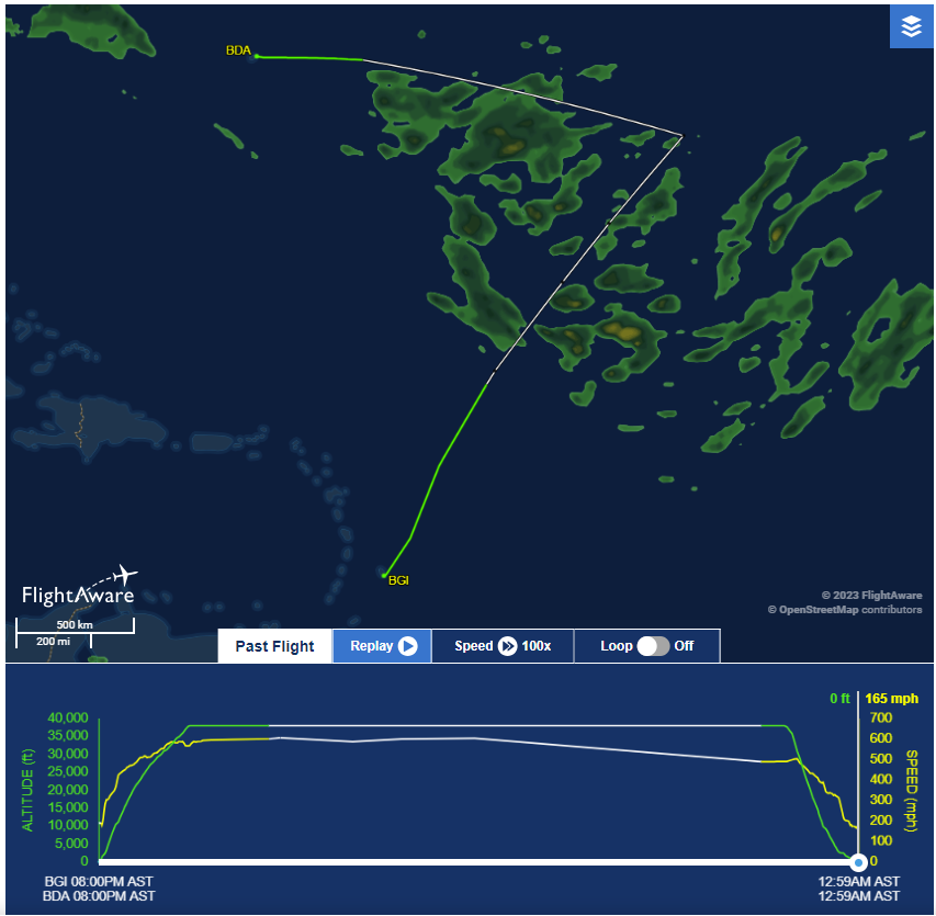
Turbulence early on 24 December on a flight (Airbus A-300) from Barbados to Manchester (Scotland) led to a diversion (to Bermuda) and hospitalization (albeit with non-life-threatening injuries) of about a dozen passengers. The graphic below shows the path of the flight with data taken from FlightAware.com. The green parts of... Read More
Turbulence early on 24 December on a flight (Airbus A-300) from Barbados to Manchester (Scotland) led to a diversion (to Bermuda) and hospitalization (albeit with non-life-threatening injuries) of about a dozen passengers. The graphic below shows the path of the flight with data taken from FlightAware.com. The green parts of the plotted path (that is, the first and last hours) come from observations, the white part of the path, including the region through convection is extrapolated. News articles on this event state (link, link, link) that turbulence occurred between 2 and 2-1/2 hours after take-off.
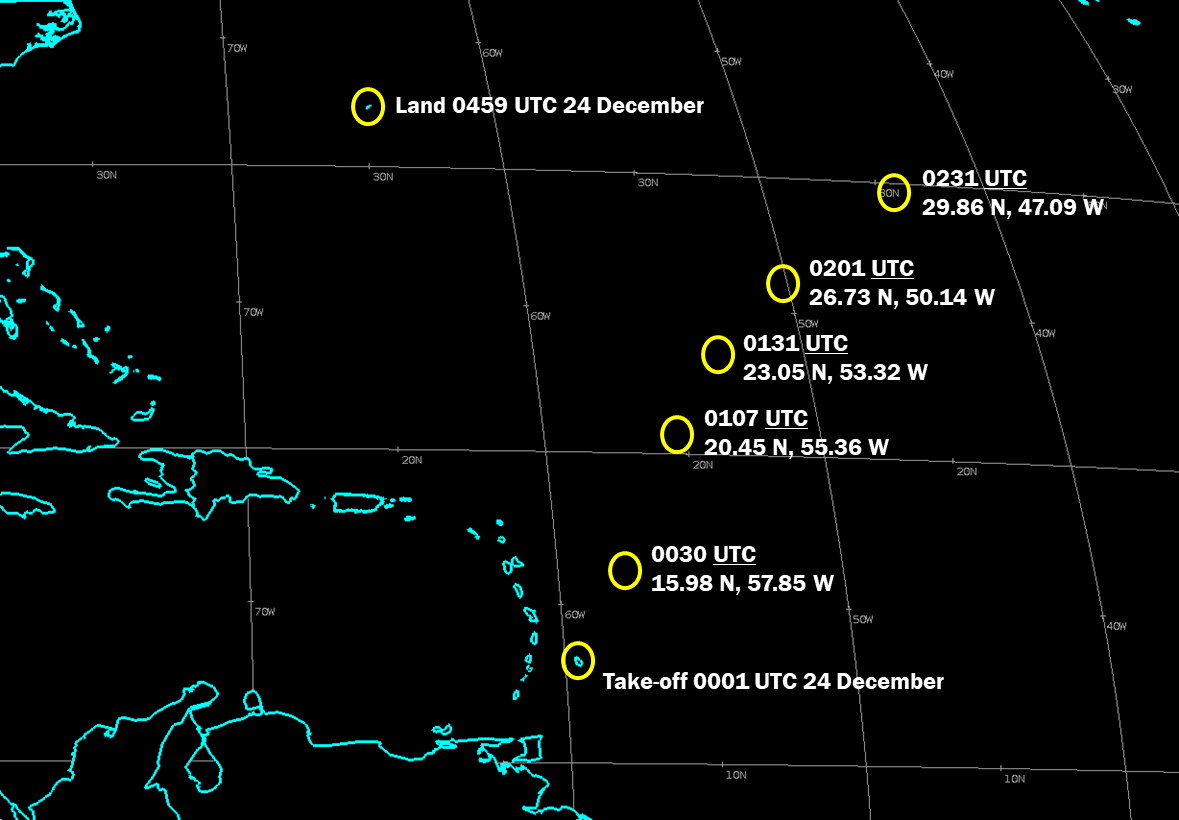
Flight path, observed (green) and estimated (white) for the Manchester-bound flight early on 24 December 2023 (Click to enlarge)Flight Path with times/locations indicated. Turbulence was observed between 2 and 2-1/2 hours after takeoff, i.e., between 0201 and 0231 UTC on 24 December 2023 (Click to enlarge)
GOES-16 Clean Window infrared (Band 13, 10.3 µm) imagery, below, shows active convection in the region where the turbulence was observed between 0200 and 0230 UTC.
GOES-16 Clean Window infrared (Band 13, 10.3 µm) imagery, 0000 to 0600 UTC on 24 December 2023 (Click to enlarge)
Upper-level water vapor (GOES-16 Band 8) imagery, below, also shows the convection in the region where turbulence occurred. (Click here to view low-level water vapor — GOES-16 Band 10 — imagery)
GOES-16 Upper-level water vapor infrared (Band 8, 6.19 µm) imagery, 0000 to 0600 UTC on 24 December 2023 (Click to enlarge)
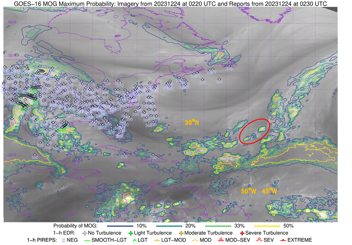
The CIMSS Turbulence product is a Machine-Learning tool that relates GOES-R imagery (and GFS estimates of lapse rates) to the probability of Moderate or Greater (MOG) turbulence. It is available online here, and is also available via an LDM feed for AWIPS. What did this product show during this event? That is shown below in an animation from 0140 to 0250 UTC on 24 December 2023. The turbulence was observed between 0200 and 0230 UTC to the south of 30oN — the latitude of northern Florida — and between 47oW and 50oW. Click here to see an annotated image from 0220 UTC.
GOES-16 Moderate-or-Greater Turbulence Probability, 0140-0250 UTC on 24 December 2023 (click to enlarge)
The plane was traversing a region where Turbulence Probability was large in places. Without a precise knowledge of where/when turbulence occurred, it’s a challenge to assess precisely how well the product performed for this event.
Perhaps GLM observations could help identify the convective feature that might have caused the convection. GLM observations between 0200 and 0240 UTC, below, bracket the reported time of the convection. If the turbulence is associated with convection, perhaps the cell near 28oN, 48oW, strong enough after all to produce lightning, was responsible.
GOES-16 GLM Flash Extent Density (1-miniute accumulations), 0200-0240 UTC on 24 December 2023; plotted on top of GOES-16 ABI Band 13 Clean Window infrared (10.3 µm) imagery every 10 minutes., (Click to enlarge)
GOES-16 (GOES-East) Nighttime Microphysics RGB and Day Snow-Fog RGB images (above) displayed the nocturnal formation — followed by the daytime dissipation — of shallow fog/stratus across snow-covered (shades of red in Day Snow-Fog RGB imagery) parts of southeastern Saskatchewan, southwestern Manitoba and northern North Dakota on 22 December 2023. With surface air temperatures dropping into the... Read More
GOES-16 Nighttime Microphysics RGB and Day Snow-Fog RGB images, from 0001 UTC to 2100 UTC on 22 December [click to play animated GIF | MP4]
GOES-16 (GOES-East)Nighttime Microphysics RGB and Day Snow-Fog RGB images (above) displayed the nocturnal formation — followed by the daytime dissipation — of shallow fog/stratus across snow-covered (shades of red in Day Snow-Fog RGB imagery) parts of southeastern Saskatchewan, southwestern Manitoba and northern North Dakota on 22 December 2023. With surface air temperatures dropping into the teens F, several METAR sites began to report freezing fog (that occasionally restricted surface visibility to near zero). Note that the shallow fog/stratus did not extend to the height of a few of the plateaus in the region (such as Turtle Mountain along the North Dakota/Manitoba border, Moose Mountain Provincial Park in Saskatchewan and Riding Mountain National Park in Manitoba).
A toggle between the GOES-16 Nighttime Microphysics RGB image at 1301 UTC and Topography (below) helped to highlight the 3 aforementioned plateau features (darker shades of tan to brown).
GOES-16 Nighttime Microphysics RGB image at 1301 UTC + Topography [click to enlarge]
The GOES-16 Cloud Thickness derived product (below) — a component of the Fog and Low Stratus suite — indicated that much of the shallow fog/stratus was generally in the 600-1200 ft thickness range.
GOES-16 Nighttime Microphysics RGB + Cloud Thickness derived product, from 0001 UTC to 1401 UTC on 22 December [click to play animated GIF | MP4]
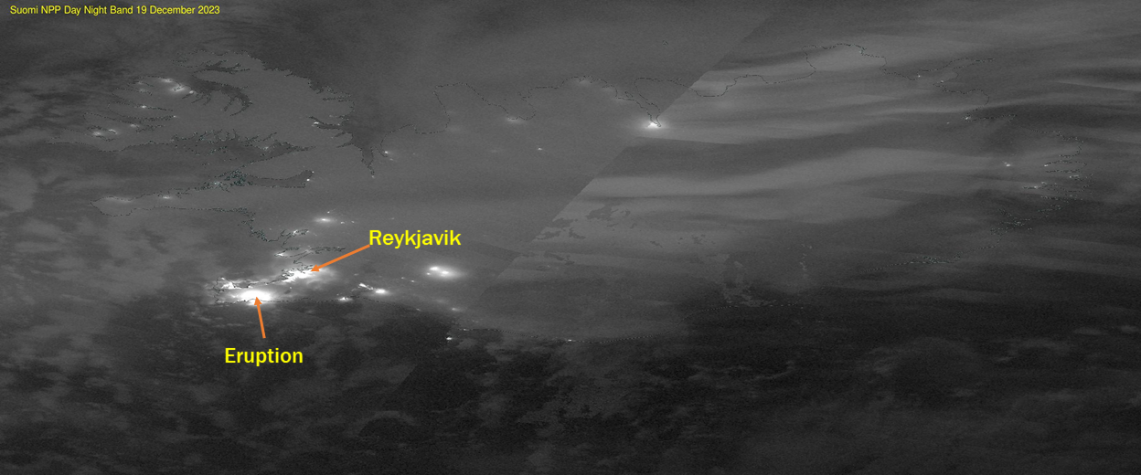
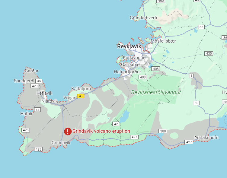
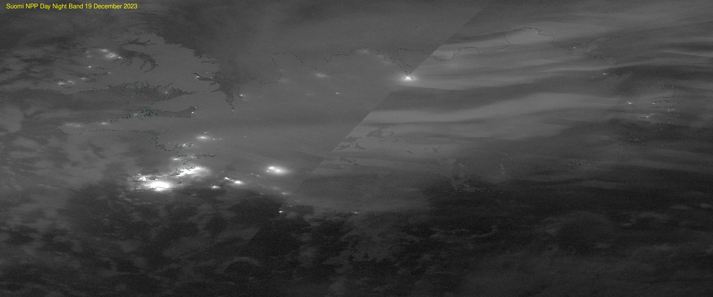
Suomi NPP Day Night Band imagery from the NASA Worldview site, had a large increase in luminance over southwest Iceland on 19 December, to the southwest of the Capitol of Reykjavik. That is shown below in the toggle of 18 December and 19 December 2023 imagery. (Click here for a map of... Read More
Suomi NPP Day Night Band imagery from the NASA Worldview site, had a large increase in luminance over southwest Iceland on 19 December, to the southwest of the Capitol of Reykjavik. That is shown below in the toggle of 18 December and 19 December 2023 imagery. (Click here for a map of southwest Iceland) Light emitted by the ongoing volcanic eruption on the Reykjanes peninsula is detected by the Day Night band sensor on VIIRS on 19 December (when Aurora Borealis are also apparent!). An annotated view of the 19 December image is also shown below.
Suomi NPP Day Night Band Visible Imagery (0.7 µm) on 18 and 19 December 2023 over Iceland (Click to enlarge)Suomi-NPP Day Night Band visible imagery, 19 December 2023 (Click to enlarge). Major light sources as indicated.
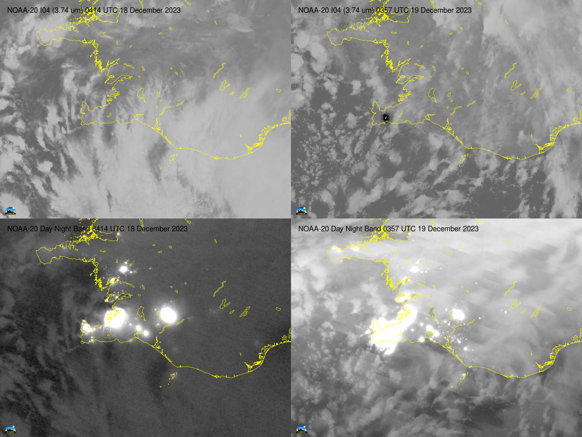
JPSS data are available via an Amazon Webservices portal (here, for NOAA-20). The CSPP software package Polar2Grid can be used to turn the SDRs available at the portal into imagery. Appropriate VIIRS-DNB-SDR and matching VIIRS-DNB-GEO files, and the VIIRS-I04-SDR and VIIRS-IMG-GEO files (a sample of which are shown below), were saved to the local machine holding the Polar2Grid software. The times of the data to select were estimated from the NOAA-20 orbit paths on 18 December and on 19 December; on the 19th, NOAA-20 flew directly over the Reykjanes peninsula.
Then, 4 different Polar2Grid calls were used to create I04 (3.74 µm) and Day Night Band visible (0.7 µm) imagery on 18 December 2023 (before the eruption) and 19 December 2023 (during the eruption), and to add maps. Those 4 images are shown below with 18 December on the left and 19 December on the right. Note the great increase in brightness and the increase in sensed temperature on 19 December!
Polar2Grid representations of NOAA-20 VIIRS I04 (3.74 µm) imagery (top) and Day Night Band visible (0.7 µm) imagery (bottom) on 18 December (left) and 19 December (right) 2023 (Click to enlarge)
In spite of frequent dense cloud cover and an oblique satellite viewng angle, a distinct hot thermal signature of the Sundhnúksgígar fissure eruption (yellow to red pixels) was occasionally apparent in GOES-16 (GOES-East) Shortwave Infrared (3.9 µm) imagery (below). Station identifier BIRK is Reykjavik Airport, and BIKF is Keflavik International Airport.
GOES-16 Shortwave Infrared (3.9 µm) images, from 2200 UTC on 18 December to 1100 UTC on 19 December (courtesy Scott Bachmeier, CIMSS) [click to play animated GIF | MP4]
Given that the fissure eruption and subsequent lava flows were occurring during the nighttime hours, the thermal signature also showed up well in GOES-16 Near-Infrared 1.61 µm and 2.24 µm imagery (below).
GOES-16 Near-Infrared “Snow/Ice” (1.61 µm, top), Near-Infrared “Cloud Particle Size” (2.24 µm, middle) and Shortwave Infrared (3.9 µm, bottom) images, from 2200 UTC on 18 December to 1100 UTC on 19 December (courtesy Scott Bachmeier, CIMSS) [click to play animated GIF | MP4]
NOAA-21 Imagery (courtesy William Straka, CIMSS), below, show that the eruption continued during the morning hours of 20 December 2023.
NOAA-21 VIIRS I04 infrared (3.74 µm) and Day Night Band visible (0.7 µm) imagery on 20 December 2023 at 0405 UTC (Click to enlarge, images courtesy William Straka, CIMSS)


