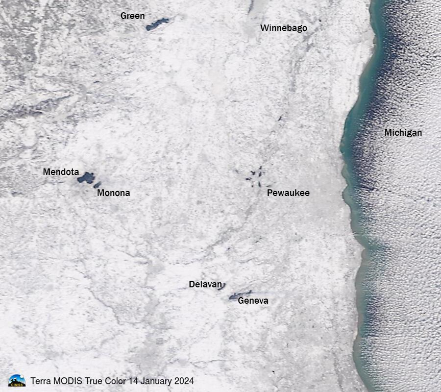
The toggle of true-color MODIS imagery above, (taken from the MODIS Today website) shows Terra MODIS imagery on 14 and 15 January 2024. The 14th was the first day of an Arctic outbreak over deep snowcover in the upper Midwest; Madison WI was at/below zero the entire day. As a consequence, many lakes that were open water on the morning of the 14th (when Terra overflew WI around 1600 UTC) were ice-covered on the morning of the 15th (when Terra overflew WI around 1630 UTC). The image below shows the 14 January imagery with some lakes named. In particular, Lake Monona and parts of Mendota froze between the 14th and 15th; many of the lakes northwest of Pewaukee Lake froze; Delavan Lake froze. Green Lake, Lake Mendota and Lake Geneva are all quite deep and therefore somewhat resistant to quick freezing, but will likely freeze over soon given the forecast.
GOES-16 animations (taken from the CSPP Geosphere site) from 14 January (above) and 15 January (below) also show the change in ice coverage.
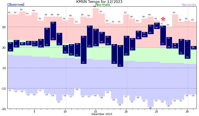
Mid-January is on the late side for lakes to freeze over Wisconsin. A warm December is to blame! Part of this is due to the ongoing Strong El Nino. In 1982-1983, a strong El Nino (as depicted at the start of this video; also shown here) similarly delayed Mendota’s freezing to mid-January.
View only this post Read Less
