If you like it, then you should put a color bar on it
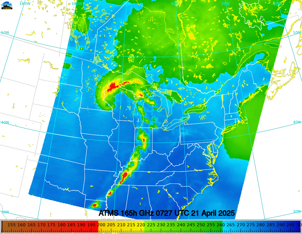
The Madison DBPS site (and other DBPS sites as detailed here) allows a user to view — in near-real time — derived MIRS imagery at different frequencies, such as the 165 GHz imagery below from NOAA-20 at 0728 UTC on 21 April 2025.
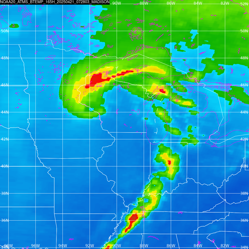
You’ll notice that (at present), a colorbar is not embedded within the image. A user who wants a colorbar, however, can easily access the data and create an image that includes brightness temperatures with a colorbar by using polar2grid — the software that is being used at the Direct Broadcast site to create the imagery above. (And yes, there are plans to embed a colorbar in the imagery at the direct broadcast site). How do you do this yourself?
You can access the data files used to create the imagery at two different locations, either at the direct broadcast site at CIMSS, i.e., the week-long storage at https://bin.ssec.wisc.edu/pub/eosdb/j01/ ; the datafiles you need are under atms, then a year/day/time, and Environmental Data Records, in this case: https://bin.ssec.wisc.edu/pub/eosdb/j01/atms/2025_04_21_111_0726/edr/ ; the files in that directory are shown below. You want the IMG file. This file contains all the data in the swath viewed by the direct broadcast antenna.
NPR-MIRS-IMG_v11r9_n20_s202504210728030_e202504210742266_c202504210807170.nc
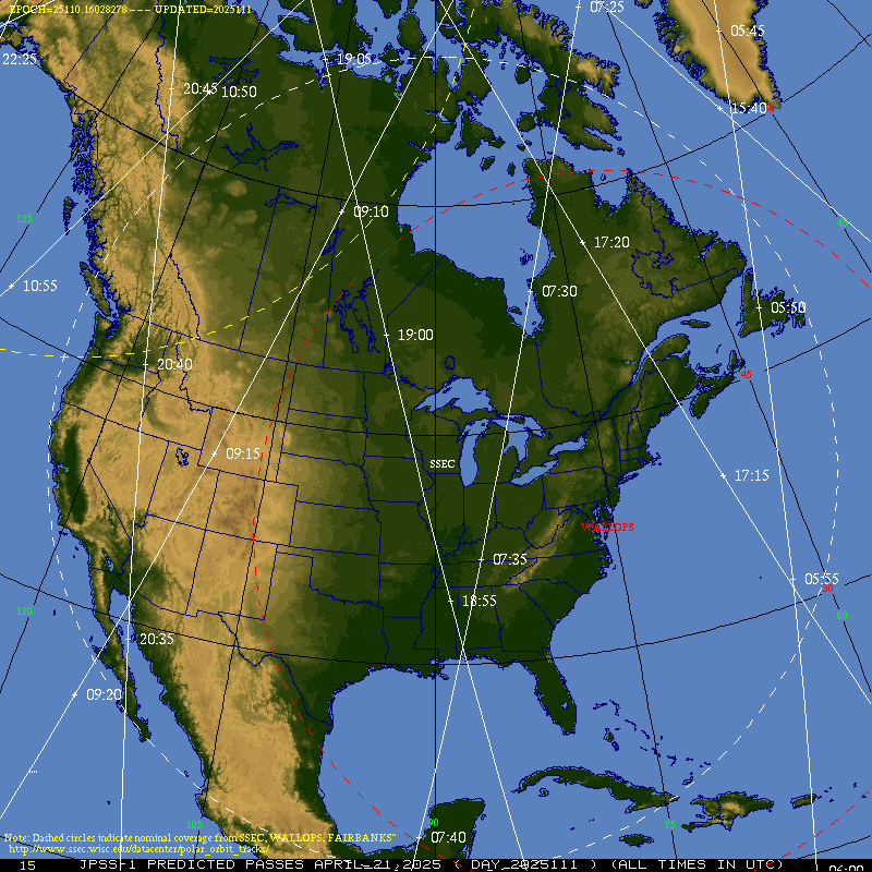
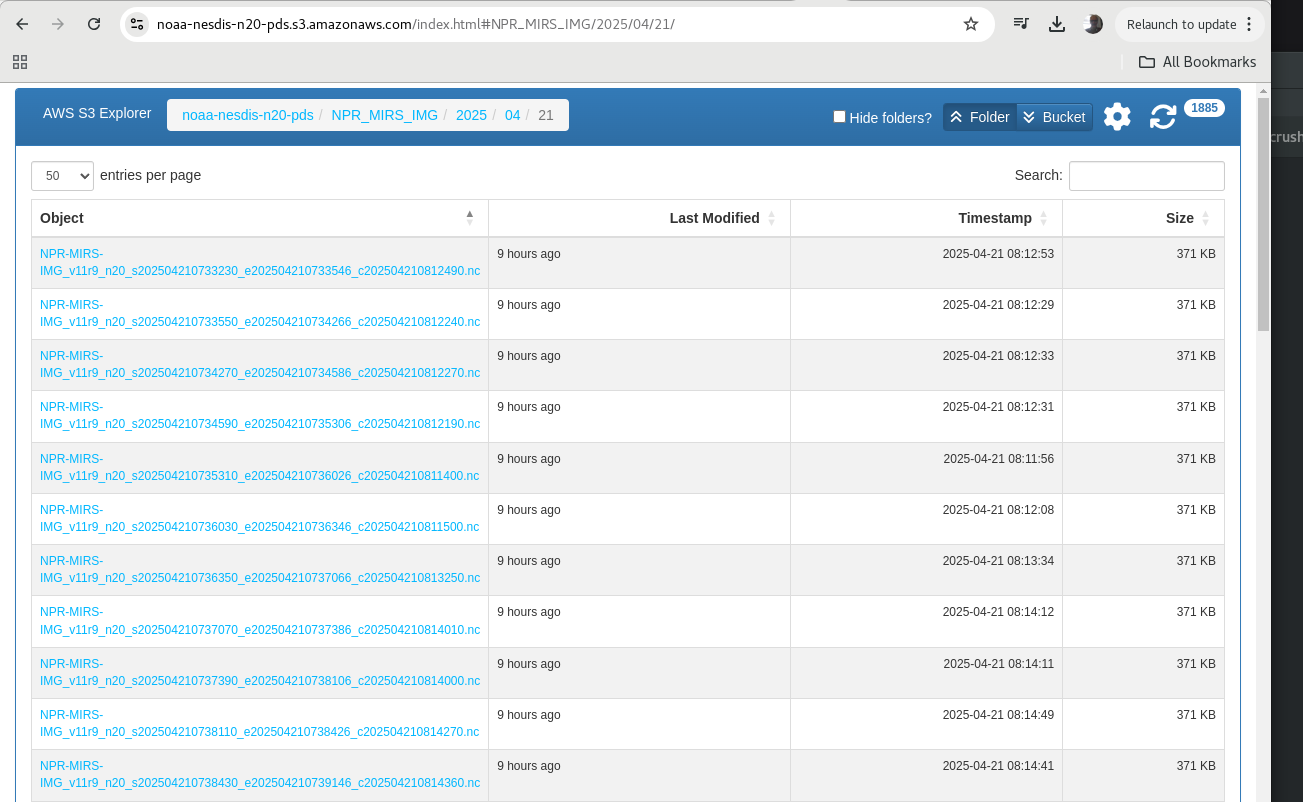
NPR-MIRS-SND_v11r9_n20_s202504210728030_e202504210742266_c202504210807170.nc You can also find similar files online at (for example) the Amazon Webservices NOAA-20 bit bucket ( https://noaa-nesdis-n20-pds.s3.amazonaws.com/index.html ). There, you can find a collection of NPR-MIRS-IMG files on 21 April 2025 ( https://noaa-nesdis-n20-pds.s3.amazonaws.com/index.html#NPR_MIRS_IMG/2025/04/21/ ); the MIRS data in these files is from smaller granules than at the Direct Broadcast site. The map below that shows NOAA-20 orbits on 21 April 2025 (from this site), means data from 0730 to 0737 UTC (approximately) is needed.
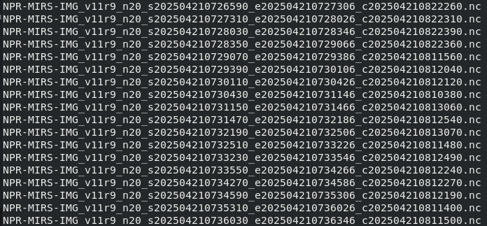
The screencapture below shows some of the files needed (of course, a simpler way to do this is to write a Python script that goes and fetches the files!). The first file on this page has data from 07:33:23.0 to 07:33:54.6 and the last file shows data from 07:38:43.0 to 07:39:14.6.
I downloaded some of these (plus others on the previous page that were from before 07:33) to my computer. The listing of the files is shown below. Now create imagery with polar2grid (free software that is downloadable here; a registration may be required. The information gathered via that registration is used only to communicate changes to users).
The first thing to do was to create a grid that approximated the one shown at the top of this blog post, using the polar2grid command p2g_grid_helper.sh. The downloaded polar2grid software went into this directory (~/Polar2Grid/polar2grid_v_3_1/) and the commands run below are being done in the bin directory just underneath the main polar2grid directory (i.e., ~/Polar2Grid/polar2grid_v_3_1/bin).
./p2g_grid_helper.sh MADISON -85.0 43.0 4000.0 -4000.0 980 760 > Madison.yamlThe command above creates a grid centered at 43.0oN, 85.0oW, with a grid spacing of 4 km (4000 m) in the E-W and N-S directions, with a size of 980×760 pixels. The script output is stored in a yaml file (that polar2grid will interpret to re-grid data).
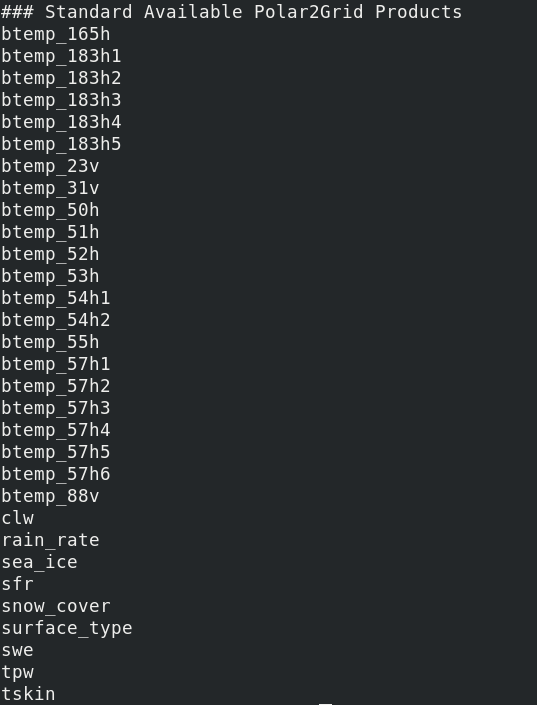
/polar2grid.sh -r mirs -w geotiff --list-products-all -f /path/to/downloaded/data/NPR-MIRS-IMG_v11r9_n20_s2025042107*.ncThe polar2grid command above lists the products that can be created. Polar2grid recognizes the data input as MIRS data — if you tell it that is the input by specifying the mirs reader : -r mirs. In addition, you can run a query about what kind of imagery can be created as shown below.
Part of that lengthy output stream from the command above is shown here. For this post I want to create 165h GHz imagery, and we’ll also create 31v and 88v GHz brightness temperatures. The polar2grid command to do that is below: the -p flag informs the software to create a list of products: brightness temperatures at 165 GHz (horizontally polarized observations), and at 88 and 31 GHz (vertically polarized observations). The data are regridded onto the ‘MADISON’ grid created above; recall that output from that grid-creation software was stored in the Madison.yaml file. All data files starting at 0700 (in this case, 072659, as listed above) will be appended by the polar2grid software). The second command adds a colormap to the created tif files.
./polar2grid.sh -r mirs -w geotiff -p btemp_165h btemp_88v btemp_31v -g MADISON --grid-configs ./Madison.yaml -f /path/to/downloaded/data/NPR-MIRS-IMG_v11r9_n20_s2025042107*

./add_colormap.sh ../colormaps/amsr2_89h.cmap noaa20_atms_btemp_*_20250421_072659_MADISON.tif
The very flexible add_coastlines shell script will (1) draw coastlines, (2) draw a latitude/longitude grid and (3) insert a colorbar. The invocation of the add_coastlines.sh is below for all three .tif files created.
./add_coastlines.sh --add-coastlines --add-borders --add-colorbar --colorbar-text-size 14 --colorbar-height 48 --add-grid --grid-D 10.0 10.0 --grid-d 10.0 10.0 --grid-text-size 12 noaa20_atms_btemp_165h_20250421_072659_MADISON.tif
./add_coastlines.sh --add-coastlines --add-borders --add-colorbar --colorbar-text-size 14 --colorbar-height 48 --add-grid --grid-D 10.0 10.0 --grid-d 10.0 10.0 --grid-text-size 12 noaa20_atms_btemp_88v_20250421_072659_MADISON.tif
./add_coastlines.sh --add-coastlines --add-borders --add-colorbar --colorbar-text-size 14 --colorbar-height 48 --add-grid --grid-D 10.0 10.0 --grid-d 10.0 10.0 --grid-text-size 12 noaa20_atms_btemp_31v_20250421_072659_MADISON.tif
The add_coastlines.sh output is a png file. The 165h GHz brightness temperature that matches the one up top (albeit on a different grid) is shown below, but now it has a colorbar!
The animation below compares the three images created, 31, 88 and 165 GHz. As expected, resolution increases as frequencies increase (because larger frequencies mean more energy). Note also how cold the 31 GHz Brightness Temperatures are over open ocean compared to 165 GHz! A conclusion can be that ocean emissivity is a function of frequency!
Note also that colorbar values are different above for 31 GHz and 88/165 GHz. These values are controlled within polar2grid in this file: polar2grid_v_3_1/etc/polar2grid/enhancements/generic.yaml ; within the file you will find (changeable!) limits for 31v, 88v, and 165h as shown below. By default, 31v is defined as 140-300, as you see above, and 88v and 165h are both defined as 150-300.

A similar method to control how CrIS data are displayed in polar2grid is in this blog post.