GOES-13 6.5 µm water vapor channel images (click image to play animation)
A major winter storm impacted much of the central Plains and the Upper Midwest regions of the US on 19 December – 20 December 2012. This storm rapidly intensified as it moved northeastward from the Texas/Oklahoma Panhandles toward southern Lake Michigan, eventually producing widespread heavy snowfall and blizzard conditions across southern Wisconsin (for additional details, see the NWS Milwaukee storm summary).Storm total snowfall smounts included 10.0 inches in Gretna, Nebraska, 14.5 inches in Alkeny, Iowa, 20.1 inches at Beaver Dam, Wisconsin, and 19.6 inches at Gaylord, Michigan. A wind gust of 71 mph was recorded at South Haven, Michigan. In addition, Chicago and Rockford in Illinois received 0.2 inches and 1.4 inches of snow, respectively, each ending their record streak of 290 consecutive days without measurable snowfall.
An animation of AWIPS images of 4-km resolution GOES-13 6.5 µm water vapor channel images (above; click image to play animation) captured the latter portion of the storm’s life cycle, from 15:15 UTC on 20 December to 02:45 UTC on 21 December. Features that were evident on the water vapor imagery included a broad warm conveyor belt with a pronounced dry slot entering the back (western) edge, and what appeared to be the development of a pair of small-scale cold conveyor belts — one that moved over the Chicago area and the southern part of Lower Michigan, and another that later moved over the northern part of Lower Michigan and Lake Huron. A well-defined deformation zone could also be seen along the western edge of the “comma head” portion of the storm.
A closer look at southern Wisconsin using 4-km resolution GOES-13 10.7 µm InfraRed (IR) images (below; click image to play animation) showed the development of colder cloud tops around -40º C (brighter green color enhancement) associated with multiple convective elements that pivoted northwestward over the area, as well as the band of colder cloud tops within the deformation zone along the rear edge of the storm system. There were a few lightning strikes with some of the stronger convective elements, producing thundersnow with enhanced snowfall rates.
GOES-13 10.7 µm IR channel images (click image to play animation)
A comparison of 1-km resolution Suomi NPP VIIRS 0.64 µm visible channel and 11.45 µm IR channel images (below) showed a more detailed view of the numerous convective elements across the region at 17:55 UTC or 12:55 PM local time — the higher spatial resolution VIIRS image displayed cloud top IR brightness temperatures as cold as -50º C (darker orange to red color enhancement).
Suomi NPP VIIRS 0.64 µm visible channel and 11.45 µm IR channel images (with METAR surface reports)
A comparison of a daytime Suomi NPP VIIRS 0.64 µm visible channel image with the corresponding false-color Red/Green/Blue (RGB) image at 19:35 UTC or 2:35 PM local time on 20 December showed that much of the northern and central Plains states had snow cover (shades of red on the RGB image); however, note that there was a large area of bare ground across the South Dakota-Nebraska border region. Even though moonlight illumination was not optimal, the Suomi NPP VIIRS 0.7 µm Day/Night Band on the following night at 07:52 UTC or 2:52 AM local time was able to show the contrast between the darker bare ground areas and the adjacent brighter areas of snow cover.
Suomi NPP VIIRS 0.64 µm visible image, False-color RGB image, and 0.7 µm Day/Night Band image
After more clouds had cleared on 21 December, another comparison of Suomi NPP VIIRS 0.64 µm visible channel and false-color RGB images at 19:16 UTC or 2:16 PM local time (below) showed better detail of the areal extent of the resulting band of fresh snow cover that stretched from Colorado eastward and northeastward into Wisconsin and Illinois. Note that the snow cover farther north across the Dakotas and Minnesota was from an earlier winter storm.
Suomi NPP VIIRS 0.64 µm visible channel image and False-color Red/Green/Blue (RGB) image
===== 22 December Update =====
A 250-meter resolution MODIS true-color image centered over Chicago (below) revealed a signature of enhanced turbidity within the nearshore waters over southern Lake Michigan on 22 December. This was a result of mixing by strong winds associated with the intensifying surface low as it passed over the area –Â wind gusts across the southern Lake Michigan region were as high as 71 mph at South Haven, Michigan and 66 mph at Michigan City, Indiana.
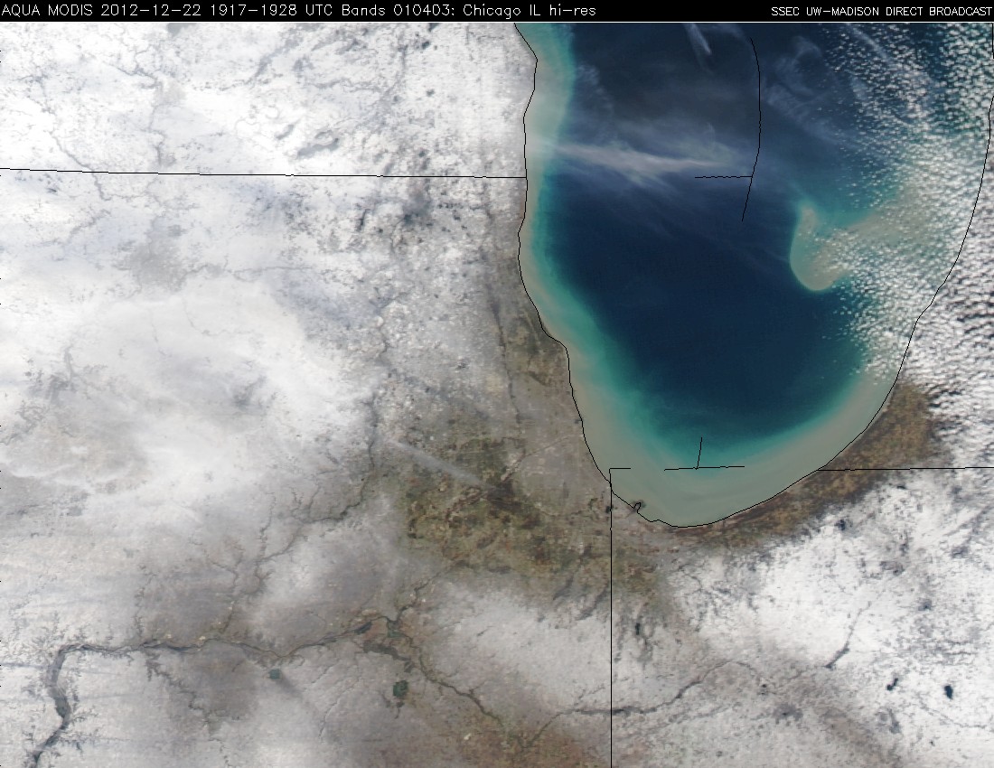
MODIS true-color Red/Green/Blue (RGB) image
View only this post Read Less