A storm forecast to produce near-record snowfalls over the Nation’s Capitol has started to move up the east coast of the United States on 22 January 2016. Snow that will fall requires two things: abundant moisture, and cold temperatures. The MIMIC Total Precipitable Water Product, shown above for the 72 hours ending at 1400 UTC on 22 January (Source) shows the circulation of the developing storm drawing moist air northward from both the Gulf of Mexico and the western Atlantic Ocean. Similarly, the toggle below shows the NESDIS Operational Blended Total Precipitable Water Product (Source, a product that ‘blends’ Total Precipitable Water observations from GPS and GOES-Sounder*). Significant moistening is apparent over the southeastern part of the United States.

*As the GOES-13 Sounder continues to be off-line due to an anomaly (Link), the principle driver of this product over the eastern US is now GPS data.

Cold air is also present. The MODIS Land Surface Temperature product from 0731 UTC on 22 January shows temperatures (in cloud-free regions) colder than -5º C southward into Virginia. Dewpoints in this region are colder than -10º C. High Pressure over the East Coast is promoting cold air damming along the Appalachians as well.

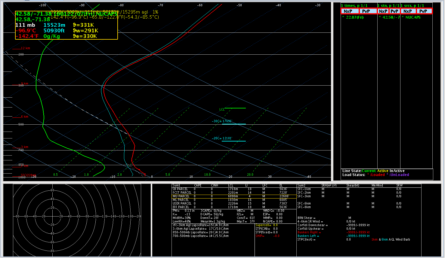
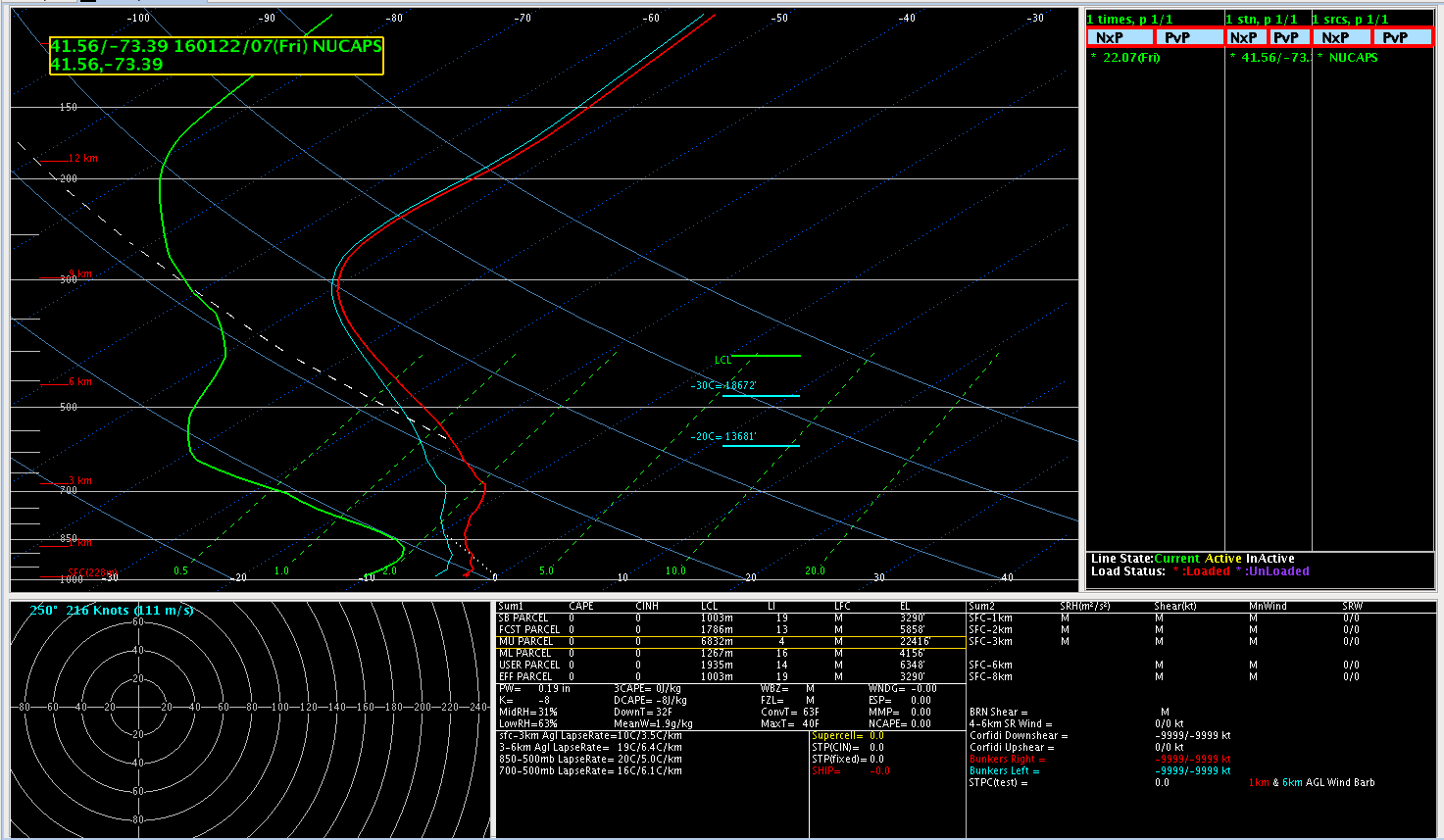
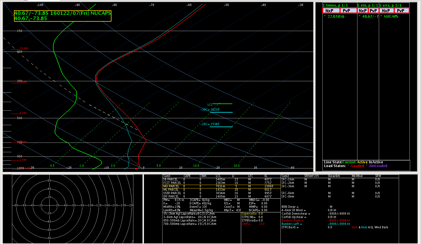
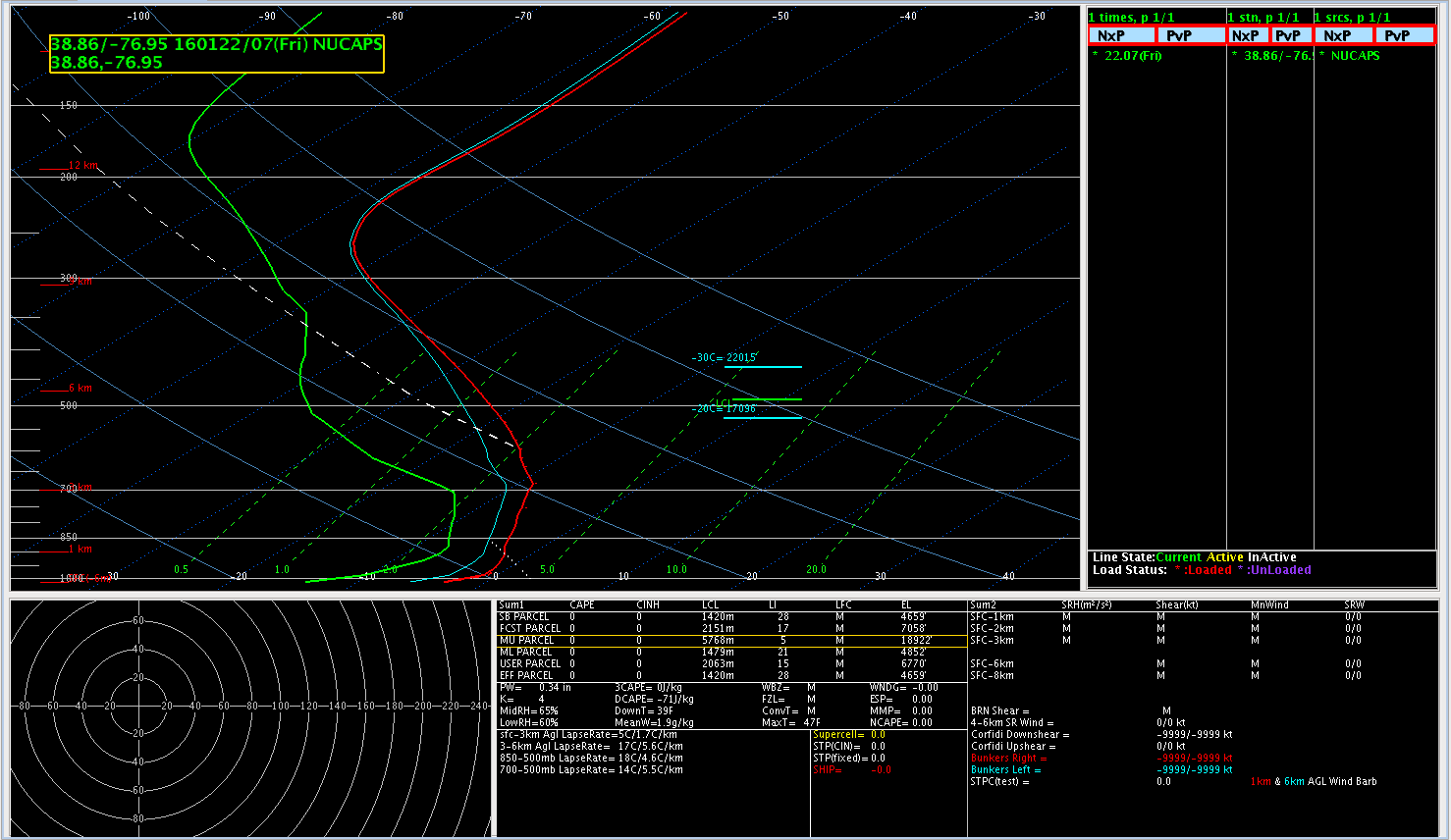
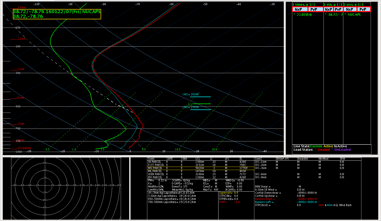
Suomi-NPP carries on board two instruments that provide vertical profiles of moisture and temperature in the atmosphere, the CrIS and the ATMS. NUCAPS Soundings combine information from those two soundings. NUCAPS Soundings sites from the early morning Suomi NPP Pass on 22 January are shown superimposed on the MODIS Land Surface Image below; five sounding sites (highlighted in red) were selected: northwest of Boston, over western Connecticut, New York City, Washington DC and central Virginia. These soundings all have common attributes: They are dry (although the vertical profiles from DC and Virginia show the most moisture: ~0.3″ of total precipitable water), they are too warm near the surface (detection of low-level inversions from satellite data is difficult) and they show lapse rates at mid-levels that suggest vigorous ascent may be possible. The 0600, 1200 and 1800 UTC Soundings from KIAD (below) also show dry air (at least initially: total precipitable water doubled from 0.24″ at 1200 UTC to 0.49″ at 1800 UTC) and steep mid-level lapse rates.

The Aqua Satellite, bearing the MODIS instrument, overflew the eastern United States shortly before 1900 UTC on 22 January 2016. MODIS samples the atmosphere at 36 different wavelengths, and selected images are shown below.

The toggle between the Visible (0.65 µm) and the ‘Snow Ice’ Channel in MODIS (1.63 µm), below, highlights regions of ice clouds. Ice particles absorb radiation with wavelength of 1.63 µm but water droplets scatter such radiation. Thus, regions in visible imagery that are white that include mostly ice crystals (or snow on the ground), for example the cirrus shield on the East Coast, will appear dark in the 1.63 µm imagery but bright in visible because clouds are highly reflective to visible light. Water-based clouds (over Mississippi, for example, or southeastern West Virginia; in fact, low clouds are apparent just to the west of the cirrus shield associated with the developing baroclinic leaf, from West Virginia southward to Savannah Georgia!) will appear bright in both channels.

MODIS also includes a channel (1.38 µm) in a region in the electromagnetic spectrum where strong water vapor absorption occurs; this channel is ideal for high cloud detection. (GOES-R will also detect radiation at this wavelength) The toggle below shows the Visible (0.65 µm), Cirrus channel (1.38 µm) and Infrared window channel (11.02 µm) from MODIS. The storm at mid-day on 22 January was producing an extensive cirrus shield that had the classic baroclinic leaf structure (a structure that was also evident in the infrared window channel).

Careful inspection of the visible and near-infrared channels from MODIS reveals transverse banding (features commonly associated with turbulence) along the western edge of the Cirrus Shield along the East Coast. The toggle below of the MODIS Water Vapor imagery (6.8 µm) shows distinct transverse banding. Pilot reports of turbulence with this system are widespread.

To better monitor the long-duration storm, the GOES-13 (GOES-East) satellite was placed into Rapid Scan Operations (RSO) mode for a 2-day period beginning at 1215 UTC on 22 January. During RSO, images are available as frequently as every 5-7 minutes, an improvement over the routine 15-minute image interval (note: the ABI instrument on GOES-R will be able to provide images as often as every minute, or even every 30 seconds). Animations of RSO Visible (0.63 µm), Water Vapor (6.5 µm), and Infrared window (10.7 µm) imagery during the daylight portion of Day 1 of the storm are shown below.

Though they lack the temporal resolution provided by geostationary satellites such as GOES, polar-orbiting satellites such as the NOAA series (with their AVHRR instrument), Terra and Aqua (with their MODIS instrument), and Suomi NPP (with the VIIRS instrument) offer imagery with significantly improved spatial resolution. Shown below is a series of AVHRR, MODIS, and VIIRS Infrared window channel images (10.8 µm, 11.0 µm, and 11.45 µm, respectively) on 22 January, with the data projected into a 1-km AWIPS-I grid. Areas with cloud-top IR brightness temperatures in the -50º to -60º C range (orange to red color enhancement) can be seen as the storm moved across the eastern US.

Excellent detail can also be seen in a series of 1-km resolution MODIS Water Vapor (6.7 µm) images spanning the 21-22 January period, shown below.

One interesting aspect to note was that the cold front associated with the intensifying storm had moved southward across the Gulf of Mexico (surface analyses), crossed the mountainous terrain of Mexico, and emerged as an area of strong gap winds over the Pacific Ocean south of Mexico (in the Gulf of Tehuantepec). The leading edge of the gap wind flow, known as a Tehuano wind (or a “Tehuantepecer”), was marked by a thin arc cloud fanning out away from the southerrn coast of Mexico, with hazy plumes of blowing dust seen streaming southward off the coast as the strong northerly winds persisted during the day.

The hazy signature of blowing dust resulting from the strong gap wind flow was even more recognizable on Suomi NPP VIIRS true-color RGB imagery, below.

GOES-13 satellite-derived atmospheric motion vector (AMV) winds, below, were showing cloud targets moving at speeds around 30-35 knots. Unfortunately, there was no good Metop ASCAT wind coverage of the Tehuano winds (as was the case for past events such as these documented here and here).

===== 23 January  Update =====

As the surface low deepened to a minimum central pressure of 983 hPa and moved northeastward just off the US East Coast (surface analyses), GOES-13 Visible (0.63 µm) images, below, showed  the moisture — with some embedded convective elements, judging from the texture and shadowing of the cloud tops — moving inland from the Atlantic Ocean north of the storm. Thundersnow was in fact reported at a number of locations. A similar animation of GOES-13 Visible images covering the daylight portions of the 22-23 January period is available here, with the entire 48-hour Infrared window channel (10.7 µm)  animation here.

Consecutive Suomi NPP VIIRS true-color RGB images at 1652 and 1828 UTC, below, provided a more detailed view of the convective elements that were moving inland north of the storm center.

===== 24 January Update =====

Shown above is a 72-hour animation of the MIMIC TPW product (from 00 UTC on 21 January to 00 UTC on 24 January), which — as mentioned at the beginning of this blog post — revealed the large amount of moisture-rich air that was drawn northward and subsequently wrapped into the storm. South of Mexico, a narrow tongue of dry air (a signature of the aforementioned Tehuano wind event) was also clearly seen, moving southwestward over the Pacific Ocean.

The entire 48-hour period of Rapid Scan Operations GOES-13 Water Vapor (6.5 µm) imagery with plots of surface weather symbols (above; also available as a large 66 Mbyte animated GIF) depicted the evolution of the storm as it moved across the Eastern US from 1215 UTC on 22 January to 1215 UTC on 24 January. The storm produced widespread heavy snowfall, areas of freezing rain and sleet, hurricane-force winds (peak gusts), and coastal flooding (WPC storm summary | NWS impacts statement | Capital Weather Gang blog) — it was ranked a Category 4 on the NESIS scale, and the 4th most intense since 1950 (NCEI overview). Features seen on the water vapor imagery included the development of a well-defined dry slot, cold conveyor belt, and elongated comma head / deformation zone that helped to produce the prolonged period of heavy snow. Interesting gravity waves were also seen within the offshore dry slot on 23 January, which appeared to be propagating westward back toward the coast. Larger-scale GOES-13 animations covering the entire 48-hour RSO period are also available [Water Vapor (6.5 µm): MP4 | animated GIF ; Infrared window channel (10.7 µm): MP4 | animated GIF].

The illumination of a Full Moon helped to provide a vivid “visible image at night” using the Suomi NPP VIIRS 0.7 µm Day/Night Band (below), highlighting the clouds associated with the departing storm along and just off the US East Coast, as well as the vast areas inland that were snow-covered. In the toggle between the corresponding Infrared window (11.45 µm) image, cloud streets due to cold air streaming southward and southeastward across the Gulf of Mexico toward Cuba were also seen.

With the arrival of daylight on the morning of 24 January, the expansive area of snow cover was very apparent on GOES-13 Visible (0.63 µm) images, shown below. Snow depth values (inches) are plotted in cyan — 12 UTC depths for the earlier images, and 18 UTC depths for the later images.  The 18 UTC snow depth values were a bit less at many locations (due to compaction and/or melting), and parts of the extreme southern and southeastern edges of the snow cover were seen to melt away during the late morning hours.

False-color Red/Green/Blue (RGB) images made using Terra MODIS Visible (0.65 µm) and Snow/Ice (1.61 µm) images, below, showed how such RGB images can be useful for the discrimination of snow/ice (shades of red) vs. supercooled clouds (shades of white). Bare ground appears as shades of cyan.

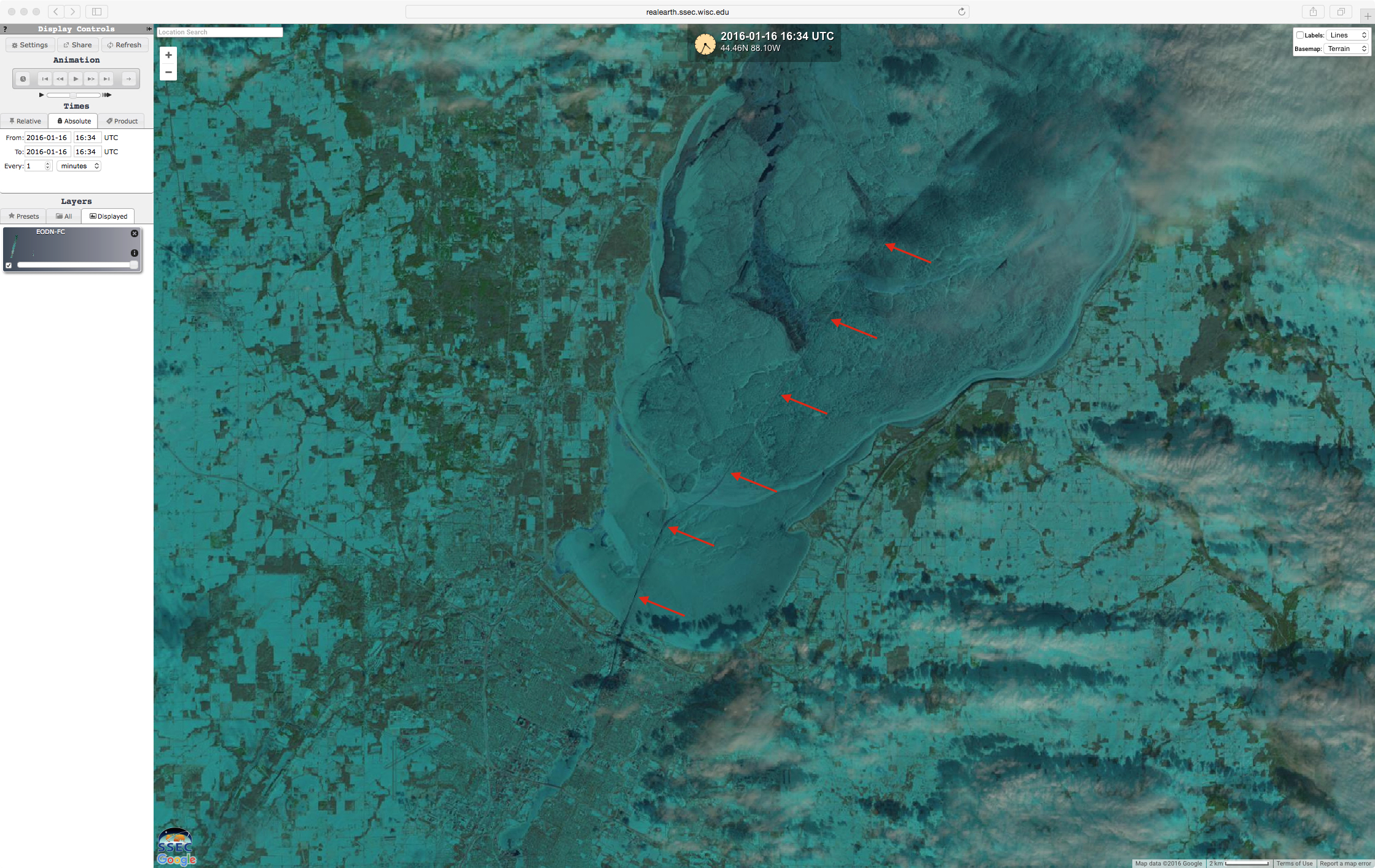
The full-resolution Terra MODIS true-color RGB images viewed using the SSEC RealEarth web map server, below, showed even better detail, including the very sharp northern edge of the snow cover from New York and Connecticut to Massachusetts.

The wider swath of the VIIRS instrument on the Suomi NPP satellite provided a good true-color vs false-color image comparison, shown below. In this particular RGB image, show/ice (and glaciated ice crystal clouds) appear as shades of cyan, while supercooled water droplet clouds appear as shades of white.

Even greater detail could be seen in a 30-meter resolution Landsat-8 false-color RGB image, centered over the Washington DC area (below). Snow and ice also appear as shades of cyan in this image — ice can be seen in parts of the Potomac and Anacostia Rivers. The partially-plowed runway network of Reagan National Airport appears at the bottom center of the image.

A close-up Landsat-8 view of the Baltimore, Maryland area (below) also showed some ice forming in a few of the rivers.

Widespread strong gusts occurred with this storm, as shown in the Table above (from the National Weather Service). The hourly animation, below, of GOES-13 Water Vapor (6.5 µm) with Wind Gusts superimposed, shows that the strongest gusts occurred as the storm’s dry slot, depicted as darker shades in the water vapor imagery and a region which is often associated with strong subsidence, was nearby.

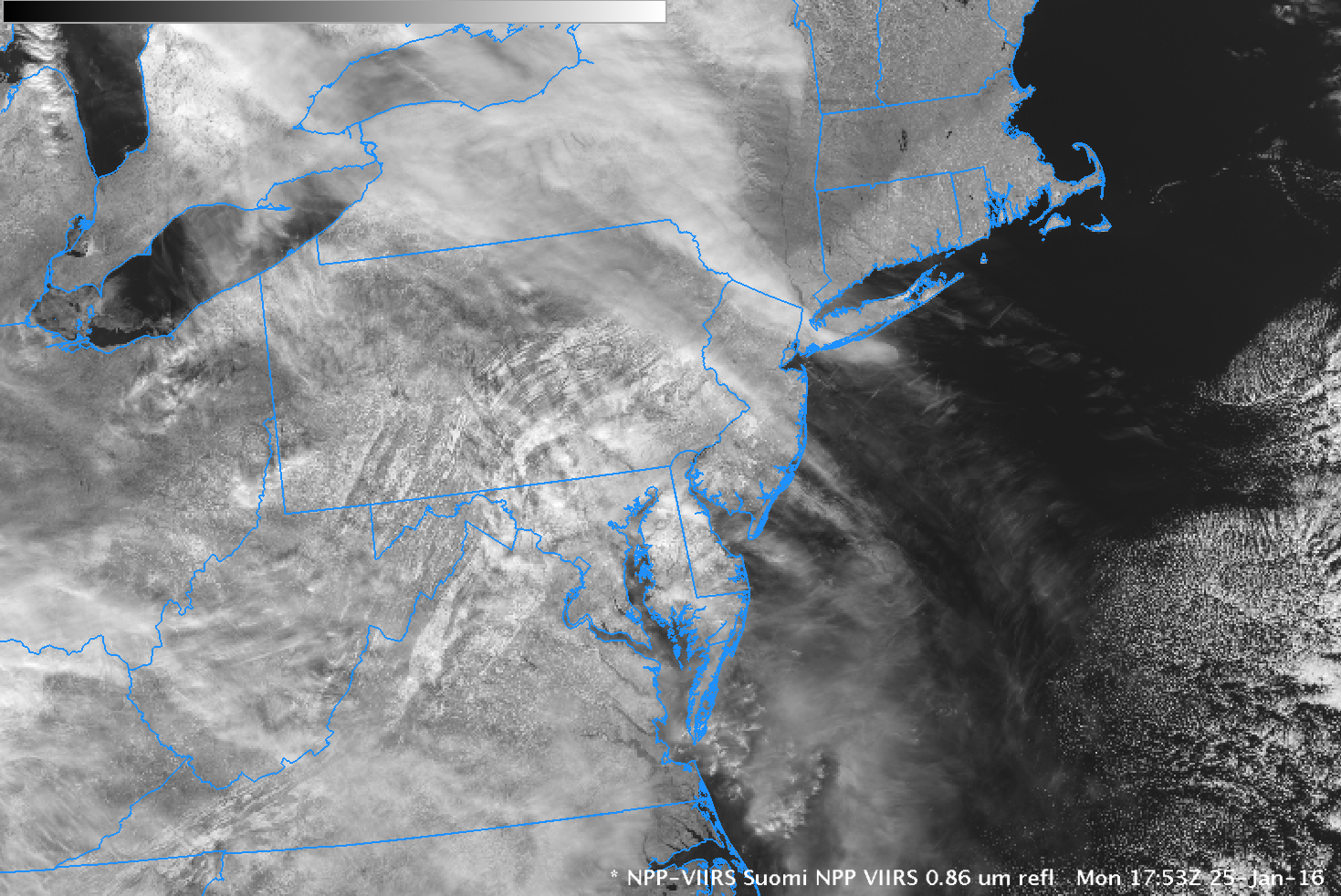
Suomi NPP VIIRS Visible and Near-Infrared imagery, below, shows the extent of the snowcover on 25 January. The benefit of multi-spectral imagery (as is available today from Suomi NPP, and will also be available from GOES-R) appears by comparing the 0.64 µm, 0.86 µm and 1.61 µm channels. For example, regions of snow vs. no snow are less distinct in the 0.86 µm (over northwest Connecticut, for example), but land/water differences are accentuated. Comparing the visible and the 1.61 µm brings out snow/ice features. The band of snow over southern New England is dark in the 1.61 µm because snow/ice absorbs radiation at that wavelength. Snow is highly reflective in the visible, however, and it appears bright white on that image. This comparison of visible and 1.61 µm can also be used to highlight ice clouds (as noted higher up in this blog post).

RGB Imagery allows a one-image perspective (vs. an image toggle) to highlight features. The RGB image from Suomi NPP VIIRS imagery (0.64 µm and 1.61 µm) below shows snow cover (shades of red) over the Northeast. In the mid-Atlantic states, thin patchy clouds are present. The brightness of these clouds in the 1.61 µm channel suggests they are composed of supercooled water droplets.

===== Added 28 January =====Rich Grumm, the SOO from the WFO in State College, discussed this storm as part of VISIT’s Satellite Chat series.

View only this post Read Less

When strong storms appear in Forecast Models, it is tempting to trace back in the atmosphere where the system originates. The water vapor animation above, from GOES-13, ends with the future East Coast Storm developing over the lower Mississippi River Valley (where it produced severe weather). The rocking animation, below, shows that the storm moved in from the Pacific Ocean on January 19th.

====================================================================================

How did the impulse traverse the Pacific Ocean? The animation above, from GOES-15, shows the system approaching the West Coast at the end of the day on Monday 18 January. It is by no means the strongest-looking system in this animation, and it has the characteristics, at 2100 UTC on 18 January, of a developing cyclone west of San Francisco. The rocking animation, below, shows that the system crossed the Pacific Basin, moving well north of Hawaii, in about two days. What did the storm do before GOES-15 could view it?

====================================================================================

The animation from Himawari-8, above (note that Himawari-8 produces Full Disk imagery every 10 minutes; GOES-13 and GOES-15 time resolution for full disk imagery is every 3 hours, and the time resolution of the Himawari-8 animation here is degraded significantly to match that of GOES-13 and GOES-15; GOES-R will have temporal resolution equivalent to Himawari), shows a series of impulses moving off the coast of Asia, with the final impulse maintaining integrity into the central Pacific (shown here at 2100 UTC on 16 January 2016; here is the view from GOES-15 at the same time). The rocking animation, below, allows for easier tracing of these impulses. The impulse that would track across the Pacific, enter North America and become a strong storm appears to be a small enhancement in the Water Vapor imagery at 0600 UTC on Friday 15 January southwest of Japan, north or Taiwan, just emerging off the coast of Asia. It can be traced back to a large low pressure system over Siberia at the beginning of the Himawari-8 animation (on 13 January).

=================================================================================

This animation strings together Himawari-8, GOES-15 and GOES-13 Water Vapor imagery from 14 January through 21 January, showing the evolution, in 3-hour steps (the native GOES-13/GOES-15 temporal resolution for Full Disk Imagery), of the system as it moves from Asia across the Pacific into North America. The images below, are annotated water vapor imagery stepping back in time showing the impulse.

View only this post Read Less

Landsat-8 imagery — with a spatial resolution of 15 to 30 meters — is available for viewing via the SSEC RealEarth web map server. An example of a swath of false-color Red/Green/Blue (RGB) imagery across the central US between the times of 1630-1640 UTC on 16 January 2016 is shown above. Snow cover and ice (as well as ice crystal clouds) appear as varying shades of cyan in this type of RGB image.  Let’s take a closer look at 3 regions along this overpass to examine some interesting features.

The northerly flow of arctic air over the still-unfrozen waters of Lake Superior was aiding the development of lake effect snow (LES) bands, some of which were moving inland over the eastern portion of the Upper Peninsula of Michigan. One of the more well-defined LES bands was seen to be moving across the Grand Marais area — a cooperative observer 10 miles south of the city reported 8.5 inches of new snow during the 24-hour period from 12 UTC on 16 January to 12 UTC on 17 January.

Looking farther to the south, an interesting feature was seen in the southern part of ice-covered Green Bay, Wisconsin (below): a channel through the ice (red arrows) had been cut by the US Coast Guard icebreaker Mackinaw during the evening of 14 January, to allow passage for a ship to unload cargo at a dock along the mouth of the Fox River (which empties into the southern end of Green Bay). Hat tip to the NWS Green Bay for providing the information on which icebreaker was involved.

Finally, a look to the southern portion of the overpass: the Mississippi River, between the states of Louisiana and Mississippi. The Landsat satellites fly over the same portion of the Earth every 17 days, so taking advantage of this fact we can visualize the profound changes in the southern Mississippi River due to the flow of large amounts of water resulting from heavy rainfall farther to the north — over the Middle Mississippi River and Ohio River Valley regions — during December 2015 (as discussed in this blog post). Water appears as darker shades of blue in these particular Landsat RGB images, aiding in the identification of areas where flooding is occurring.

View only this post Read Less

Subtropical Storm Alex (NHC advisory archive) formed in the far eastern Atlantic Ocean on 13 January 2016. Animations of GOES-13 (GOES-East) 0.63 µm Visible (above) and 10.7 µm Infrared images (below) showed the initial evolution and northeastward motion of the storm. Alex is only the 4th known January tropical or subtropical storm to have formed in the Atlantic since the historical record began in 1851.

===== 14 January Update =====

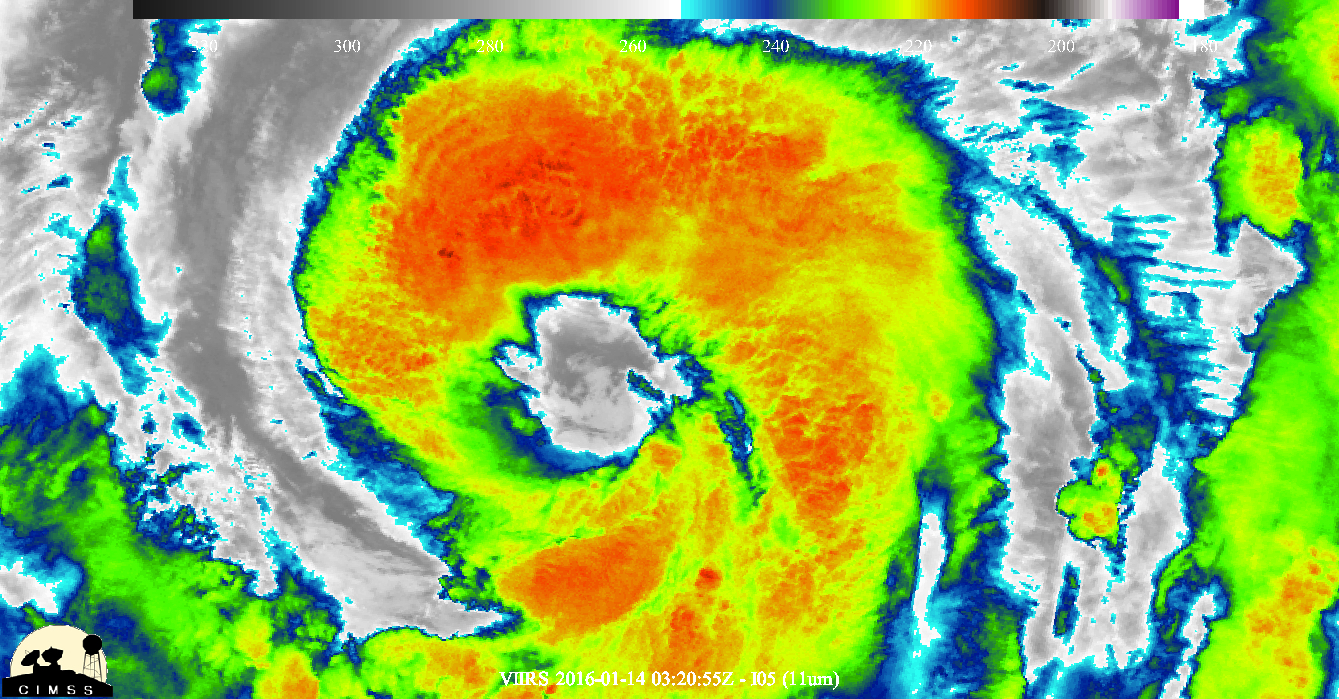
A comparison of Suomi NPP VIIRS Infrared (11.45 µm) and Day/Night Band (0.7 µm) images at 0320 UTC (below) showed the well-defined eye of Alex. With the Moon in the Waxing Crescent phase (at 30% of Full) there was enough illumination to demonstrate the “visible image at night” capability of the Day/Night Band. A magnified version of the Infrared image showing the eye can be seen here.

As of 15 UTC on 14 January, Alex had made the transition from subtropical storm to Category 1 hurricane (eastern Atlantic Ocean surface analyses). GOES-13 Infrared (10.7 µm) images (below) showed the well-defined eye that had formed. Alex became the first known hurricane to form in the Atlantic Ocean since 1938, and only the second hurricane on record to from north of 30ºN latitude and east of 30ºW longitude.

A DMSP-16 SSMIS Microwave (85 GHz) image (below) revealed the eye structure at 1653 UTC.

===== 15 January Update =====

While still classified as a hurricane, Alex was undergoing a weakening trend as it approached the Azores Islands during the early morning hours on 15 January. GOES-13 Infrared (10.7 µm) images (below) showed a strong convective band that produced a brief period of heavy rain at Ponta Delgata and Lajes Acores several hours prior to the passage of the eye of Alex (which occurred in the 11-14 UTC time frame — and Alex was downgraded at that point to a Tropical Storm). At Ponta Delgata a peak wind gust of 50 knots was recorded at 1130 UTC.

ISS-Rapidscat surface scatterometer winds (below) showed the center of circulation of Alex just south of the Azores Islands at 1118 UTC.

===== 16 January Update =====

Using a long animation of GOES-13 Water Vapor (6.5 µm) images covering the 06-16 January period (below; also available as a large 165-Mbyte animated gif), the origination of Hurricane Alex could be traced back to a strong baroclinic mid-latitude cyclone that rapidly intensified off the southeast coast of the US on 07 January.

The origin and motion of Alex could also be identified using the satellite-derived atmospheric motion vector 850 hPa Relative Vorticity product (below). A region of lower-tropospheric vorticity over Cuba on 06 January began moving northeastward across the Bahamas, then eastward across the Atlantic Ocean on 07 January.

For another perspective on the history of the development of Alex, see this article from The Weather Channel.

View only this post Read Less