A plot of the Advanced Dvorak Technique for Typhoon Lan (above) showed that the tropical cyclone underwent a period of rapid intensification during the 00-12 UTC period on 20 October 2017.A 24-hour animation of Himawari-8 rapid-scan (2.5 minute interval) Infrared Window (10.4 µm) images (below) revealed the development of a very large... Read More
![Advanced Dvorak Technique (ADT) plot for Typhoon Lan [click to enlarge]](https://cimss.ssec.wisc.edu/satellite-blog/wp-content/uploads/sites/5/2017/10/Lan_adt.gif)
Advanced Dvorak Technique (ADT) plot for Typhoon Lan [click to enlarge]
A plot of the
Advanced Dvorak Technique for Typhoon Lan
(above) showed that the tropical cyclone underwent a period of rapid intensification during the 00-12 UTC period on 20 October 2017.
A 24-hour animation of Himawari-8 rapid-scan (2.5 minute interval) Infrared Window (10.4 µm) images (below) revealed the development of a very large eye during the 20 October/06 UTC to 21 October/06 UTC period.
![Himawari-8 Infrared Window (10.4 µm) images [click to play MP4 animation]](https://cimss.ssec.wisc.edu/satellite-blog/wp-content/uploads/sites/5/2017/10/960x1280_AHIM08_B13_HIM08_IR_LAN_20OCT2017_2017293_170215_0001PANEL.GIF)
Himawari-8 Infrared Window (10.4 µm) images [click to play MP4 animation]
A nighttime comparison of Suomi NPP VIIRS Day/Night Band (0.7 µm) and Infrared Window (11.45 µm) images at 1700 UTC or 2:00 AM kocal time
(below; courtesy of William Straka, CIMSS/SSEC) provided a good visualization of the “stadium effect” — an eye that was more narrow at the surface, with a larger diameter at higher altitudes. A packet of mesospheric airglow waves (
reference) was also evident on the Day/Night Band image, propagating south-southeastward away from the eye.
![Suomi NPP VIIRS Day/Night Band (0.7 µm) and Infrared Window (10.4 µm) images [click to enlarge]](https://cimss.ssec.wisc.edu/satellite-blog/wp-content/uploads/sites/5/2017/10/171020_1700utc_suomi_npp_viirs_InfraredWindow_DayNightBand_Typhoon_Lan_anim.gif)
Suomi NPP VIIRS Day/Night Band (0.7 µm) and Infrared Window (10.4 µm) images [click to enlarge]
A 2-panel comparison of Himawari-8 Visible (0.64 µm) and Infrared Window (11.45 µm) images
(below) showed the eye of Lan after it attained Super Typhoon status at 18 UTC on 20 October. Mesovortices could be seen within the eye on the rapid-scan images.
![Himawari-8 Visible (0.64 µm, left) and Infrared Window (10.4 µm, right) images [click to play MP4 animation]](https://cimss.ssec.wisc.edu/satellite-blog/wp-content/uploads/sites/5/2017/10/960x640_AHIM08_B313_HIM08_VIS_IR_LAN_20OCT2017_2017294_030215_0002PANELS.GIF)
Himawari-8 Visible (0.64 µm, left) and Infrared Window (10.4 µm, right) images [click to play MP4 animation]
A large amount of moisture was associated with this tropical cyclone, as depicted by hourly images of the
MIMIC Total Precipitable Water product
(below) — note the large area with TPW values of 70 mm or greater
(light violet color enhancement).
![MIMIC Total Precipitable Water product [click to play animation]](https://cimss.ssec.wisc.edu/satellite-blog/wp-content/uploads/sites/5/2017/10/wpac20171021.120000_tpw.png)
MIMIC Total Precipitable Water product [click to play animation]
A TPW value of 72.5 mm (2.87 inches) was derived from the Minamidaitojima, Japan rawinsonde data at 12 UTC on 21 October
(below). Minamidaitojima is the largest island in the Daito Islands group southeast of Okinawa, Japan — this station was just to the northeast of Lan around 12 UTC.
![Rawinsonde data from Minamidaitojima, Japan [click to enlarge]](https://cimss.ssec.wisc.edu/satellite-blog/wp-content/uploads/sites/5/2017/10/171021_47945_ROMD_RAOBS.GIF)
Rawinsonde data from Minamidaitojima, Japan [click to enlarge]
View only this post
Read Less
![GOES-1 Visible image at 1645 UTC on 25 October 1975 [click to enlarge]](https://cimss.ssec.wisc.edu/satellite-blog/wp-content/uploads/sites/5/2019/10/19751025_1645utc_goes1_visible.jpg)
![GOES-1 Visible image, 0700 UTC on 10 April 1979 [click to enlarge]](http://cimss.ssec.wisc.edu/goes/fd/1970s/FD_GOES-1_VIS_MED_BIG_NOMAP_10-Apr-1979_0700_UTC_4by4.JPG)
![GOES-1 Visible (0.65 µm) image, 0930 UTC on 01 January 1979 [click to enlarge]](https://cimss.ssec.wisc.edu/satellite-blog/wp-content/uploads/sites/5/2017/10/FD_GOES-1_VIS_MED_NOMAP_01-Jan-1979_0930_UTC.JPG)
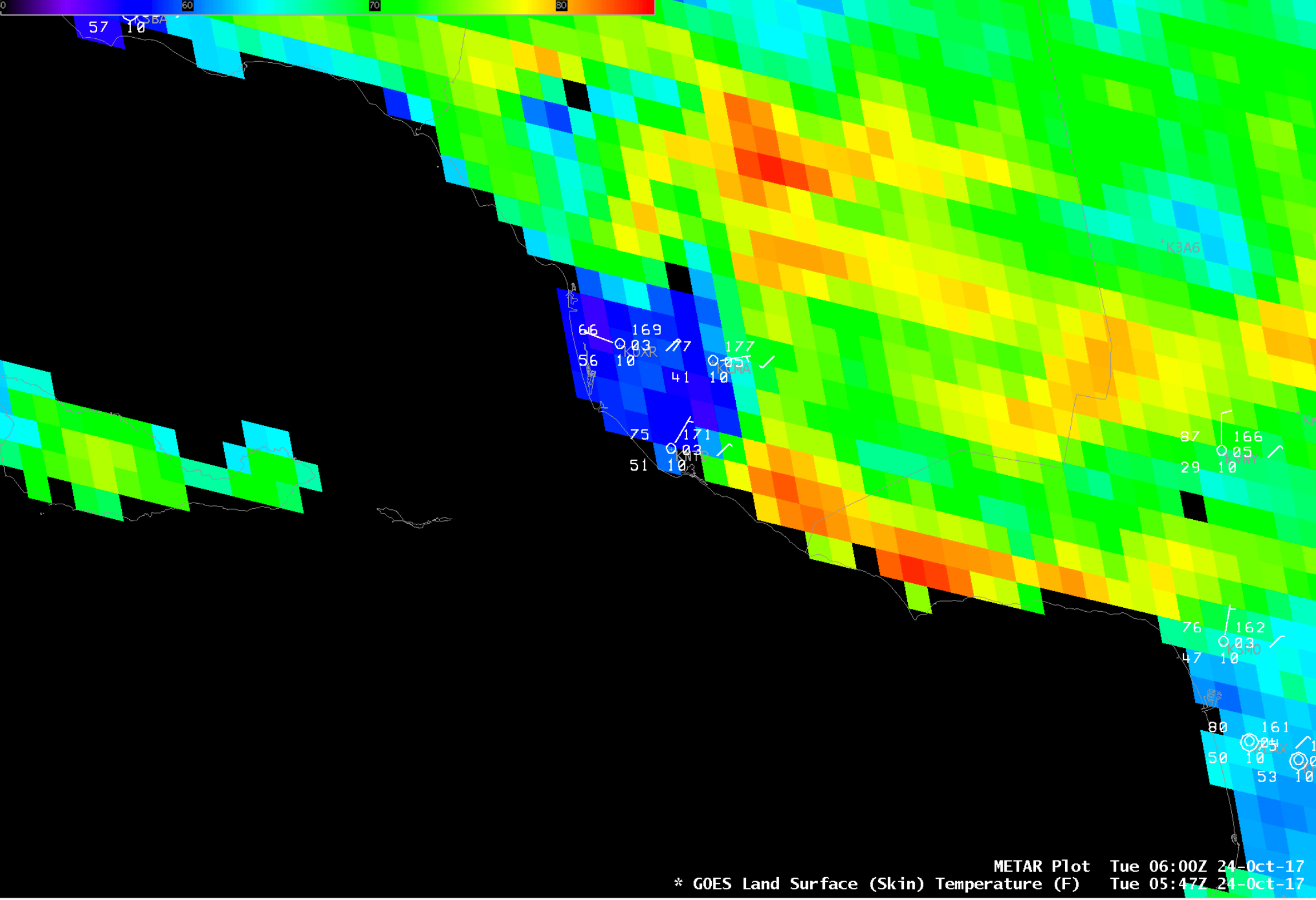
![GOES-16 Land Surface Temperature product, with hourly surface reports plotted in white [click to enlarge]](https://cimss.ssec.wisc.edu/satellite-blog/wp-content/uploads/sites/5/2017/10/LST-VenturaCounty-Overnight.gif)
![Terra and Aqua MODIS Land Surface Temperature product [click to enlarge]](https://cimss.ssec.wisc.edu/satellite-blog/wp-content/uploads/sites/5/2017/10/171024_modis_land_surface_temperature_SoCal_anim.gif)
![GOES-16 Shortwave Infrared (3.9 µm) images [click to play MP4 animation]](https://cimss.ssec.wisc.edu/satellite-blog/wp-content/uploads/sites/5/2017/10/SantaAna_B07_COU_CONUS_logos_800x1200_B7_2017297_080220_0001PANEL_00049_labels.gif)
![MIMIC Total Precipitable Water product [click to play animation]](https://cimss.ssec.wisc.edu/satellite-blog/wp-content/uploads/sites/5/2017/10/171020-22_mimic_tpw_Lan_anim.gif)


