GOES-19 True-Color animations on 5 May and 4 May 2025 (from the CSPP Geosphere site) show a circulation cut off from the main westerlies and slowly meandering across the Ohio River Valley. The system has become a bit more symmetric on the 5th as it separates more completely from the front along the east coast. A MIMIC Total Precipitable Water animation for the 24 hours ending 1600 UTC on 5 May, below, shows the system surrounded by relatively dry air.

Advected Layer Precipitable Water (ALPW) fields, below, from ca. 0300 UTC 4 May 2025 and 1500 UTC 5 May 2025 (from this site) shows that the system is stacked in the vertical and moving very very slowly.

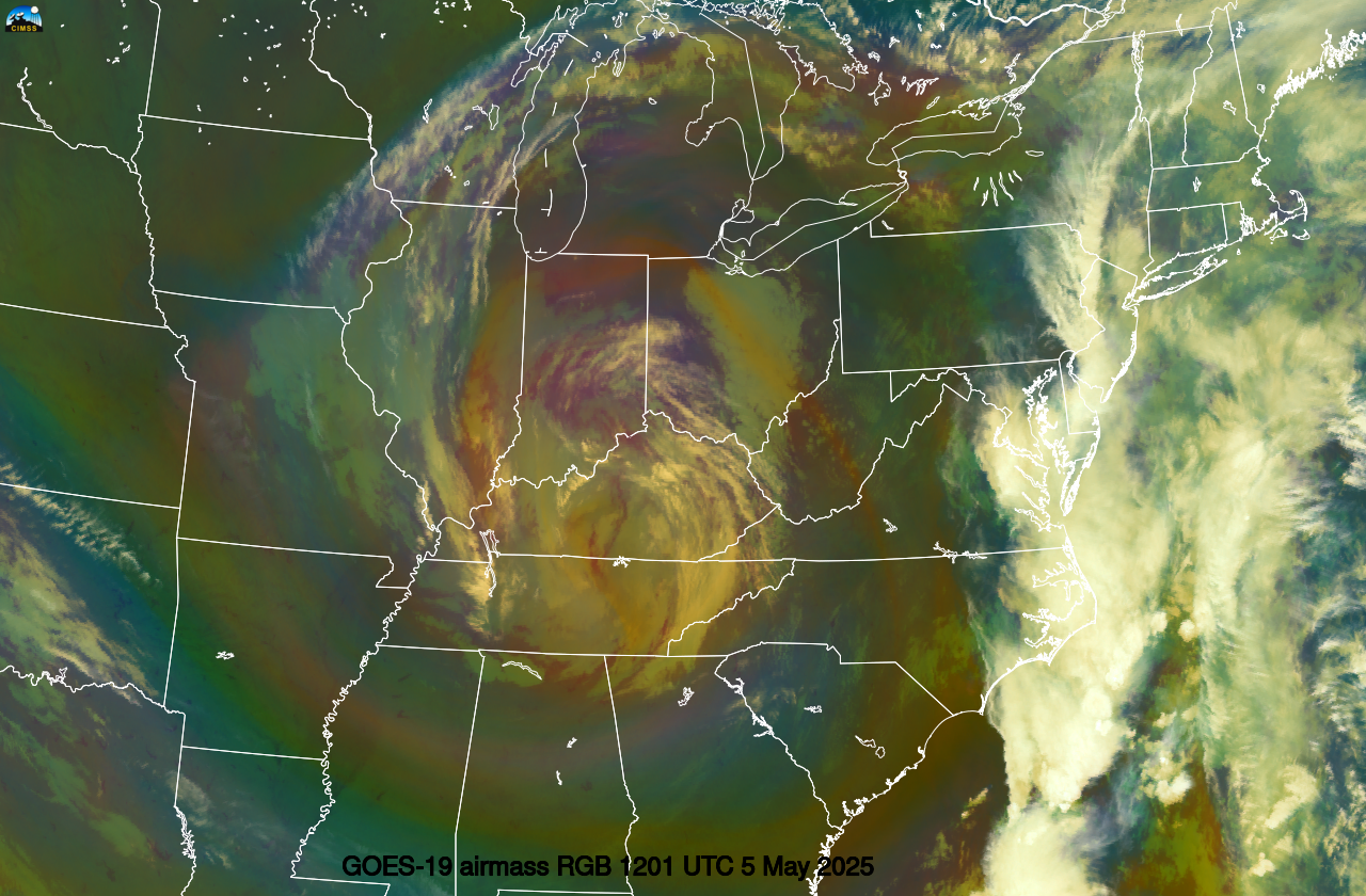
Airmass RGB shows the system drifting across northern Kentucky in the 38 hours ending at 1400 UTC 5 May 2025. It is spawning clouds and showers over a large portion of the eastern United States as the storm meanders, as shown in this radar animation from here.

The animation below shows the evolution of the surface system from 2100 UTC 3 May through 1200 UTC 5 May 2025.

500-mb heights on 5 May 2025 (below, at 0000 and 1200 UTC), clearly show the system over Kentucky. A system over the southwestern United States is poised to kick the storm over the Ohio River valley to the east.

View only this post Read Less

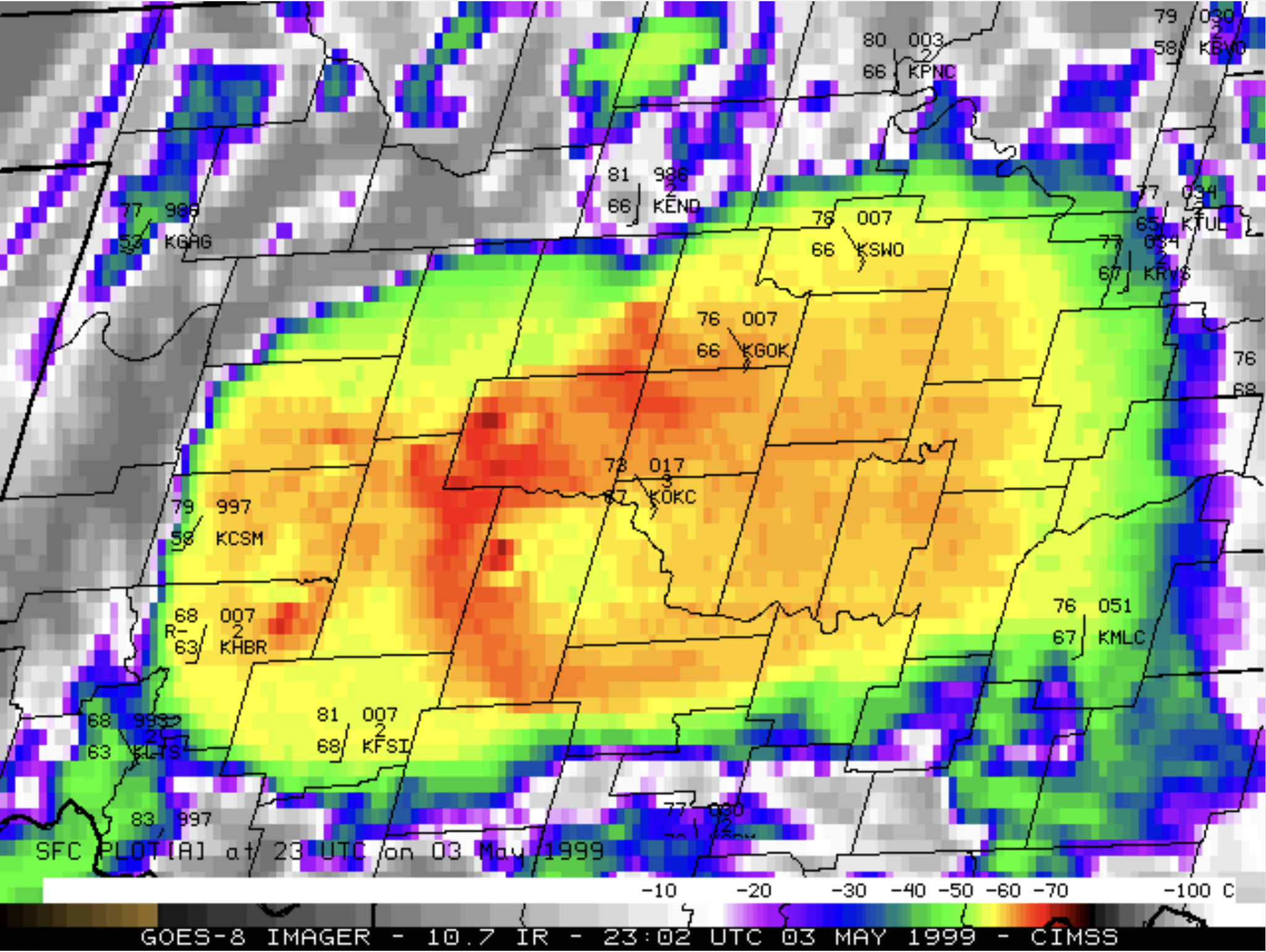
A significant outbreak of tornadoes occurred across Oklahoma and Kansas during the afternoon and evening hours on 03 May 1999 — and hail as large as 4.50 inches in diameter was reported in parts of Texas and Oklahoma (Storm Reports). NWS damage surveys indicated that widespread F4 and F5 tornado damage occurred. NOAA GOES-8 Visible images (above) and Infrared images (below) centered on Oklahoma City (KOKC) showed the explosive development of convection across southwestern Oklahoma after 2045 UTC. Several overshooting tops were evident in the visible imagery, and Enhanced-V cloud-top signatures were seen in the Infrared imagery.

A toggle between GOES-8 Visible and Infrared images at 2302 UTC (below) displayed distinct overshooting top and Enhanced-V signatures associated with the supercell thunderstorm that was southwest of Oklahoma City — about 50 minutes prior to the first tornado reports in the Newcastle area (10 miles south of KOKC).

GOES-8 Water Vapor images (below) showed the approach of an upper-level shortwave trough during the afternoon hours.

Strong upper-level divergence indicated that forcing for synoptic-scale lift was likely being enhanced as a jet streak moved over Oklahoma (below).

GOES-8 Sounder lifted index (LI) and total precipitable water (PW) derived products are shown below. During the morning hours preceding convective development, a trend of rapid destabilization was evident from central Texas into Oklahoma (LI’s decreased to -8 C and lower, red enhancement); in addition, the moisture gradient appeared to increase slightly along the dryline that was located across western Oklahoma.

AERI retrieval data was combined with GOES-8 Sounder data to produce Skew-t/log-p thermodynamic diagrams for the atmosphere over Purcell (in south-central Oklahoma) at 1934 UTC and 2043 UTC UTC (below), during the hour preceding convective development. Note how the low-level “capping inversion” near 850 hPa was eroded, allowing organized surface-based updrafts to ascend above the level of free convection. In that 1-hour period, the CAPE increased from 4111 to 4681 J/kg, and the lifted index (LI) decreased from -7.48 to -8.22 C; convective inhibition (CIN) decreased from -259 to -69 J/kg.

A time series of convective indices for the 4 Oklahoma AERI + GOES Sounder sites (below) showed the trend of rapid destabilization during the afternoon hours leading up to the development of supercell convection.

View only this post Read Less

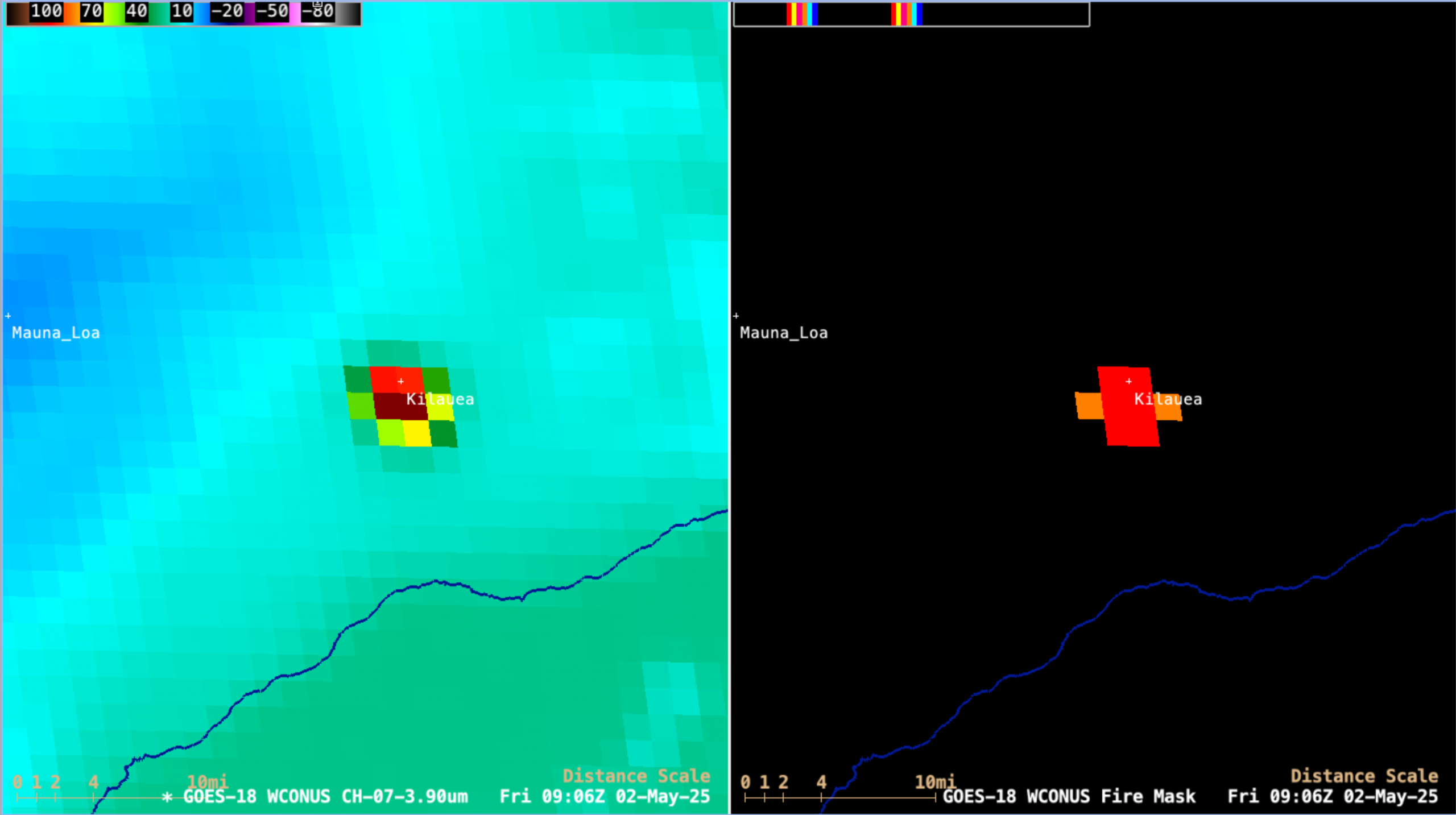
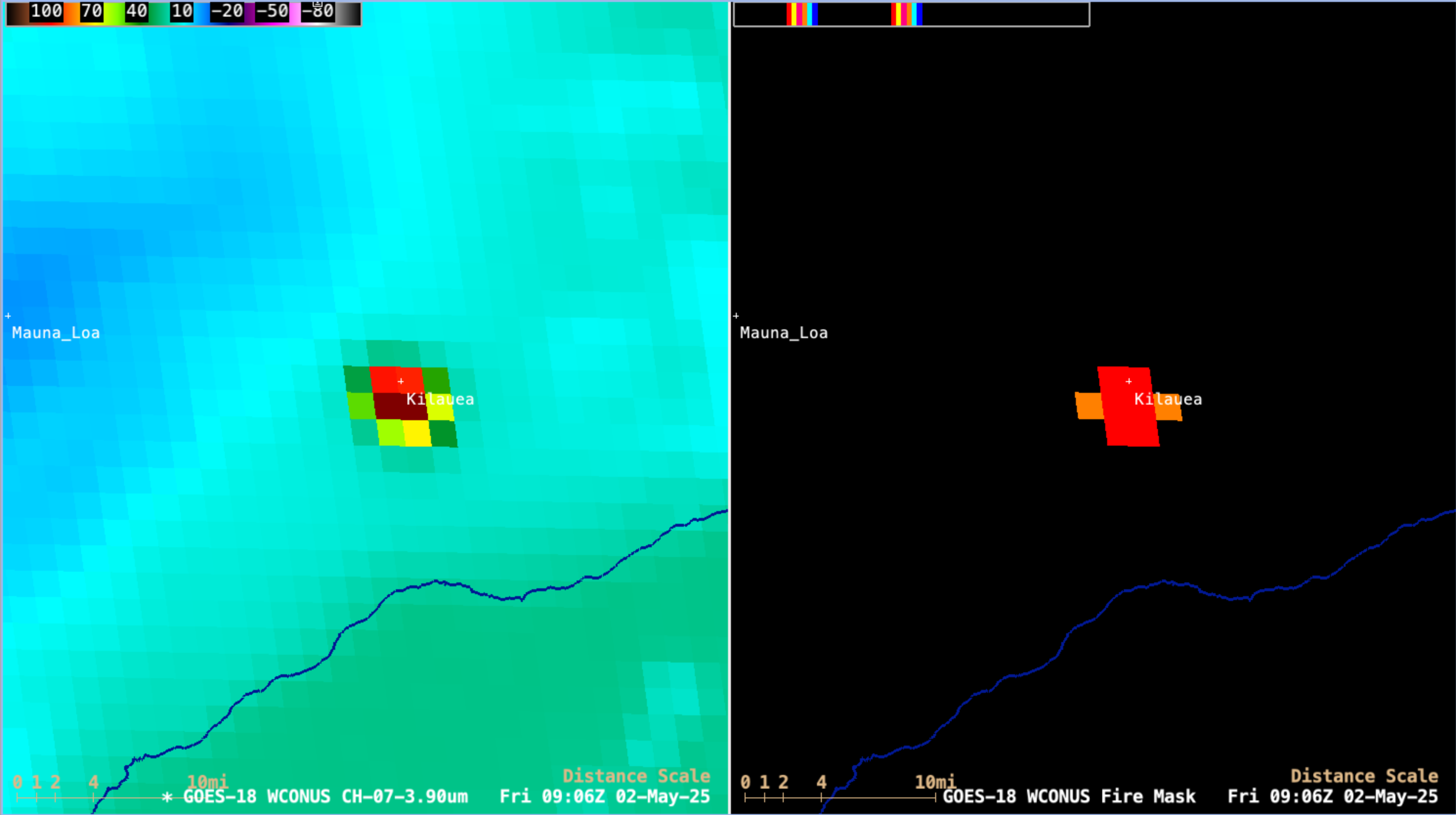
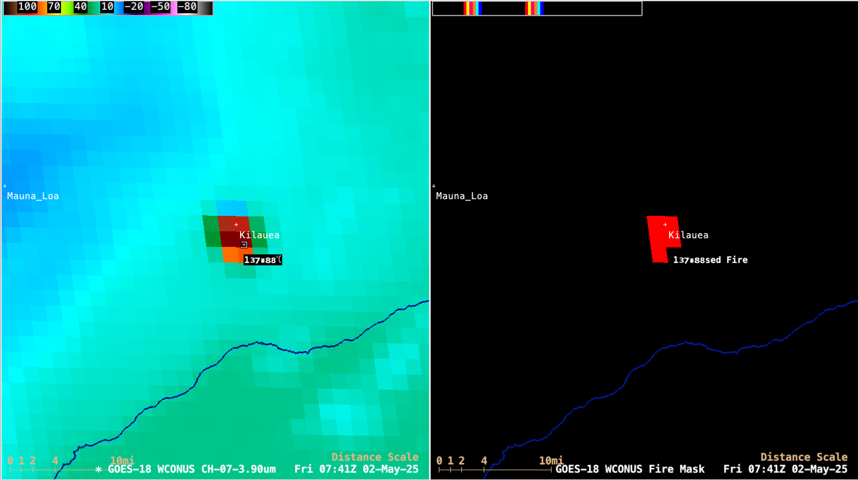
5-minute CONUS Sector GOES-18 (GOES-West) Shortwave Infrared (3.9 µm) and Fire Mask derived product images (above) displayed a pronounced thermal signature associated with Episode 19 of the ongoing eruption in the Halema’uma’u crater (located within the Kilauea summit caldera) on the Big Island of Hawai’i, which began around 0728 UTC on 02 May 2025. Shortwave Infrared 3.9 µm brightness temperatures exhibited values of 137.88ºC — the saturation temperature of GOES-18 ABI Band 7 detectors — for several hours, beginning at 0741 UTC. This prolonged multi-episode Kilauea eruption began on 23 December 2024.

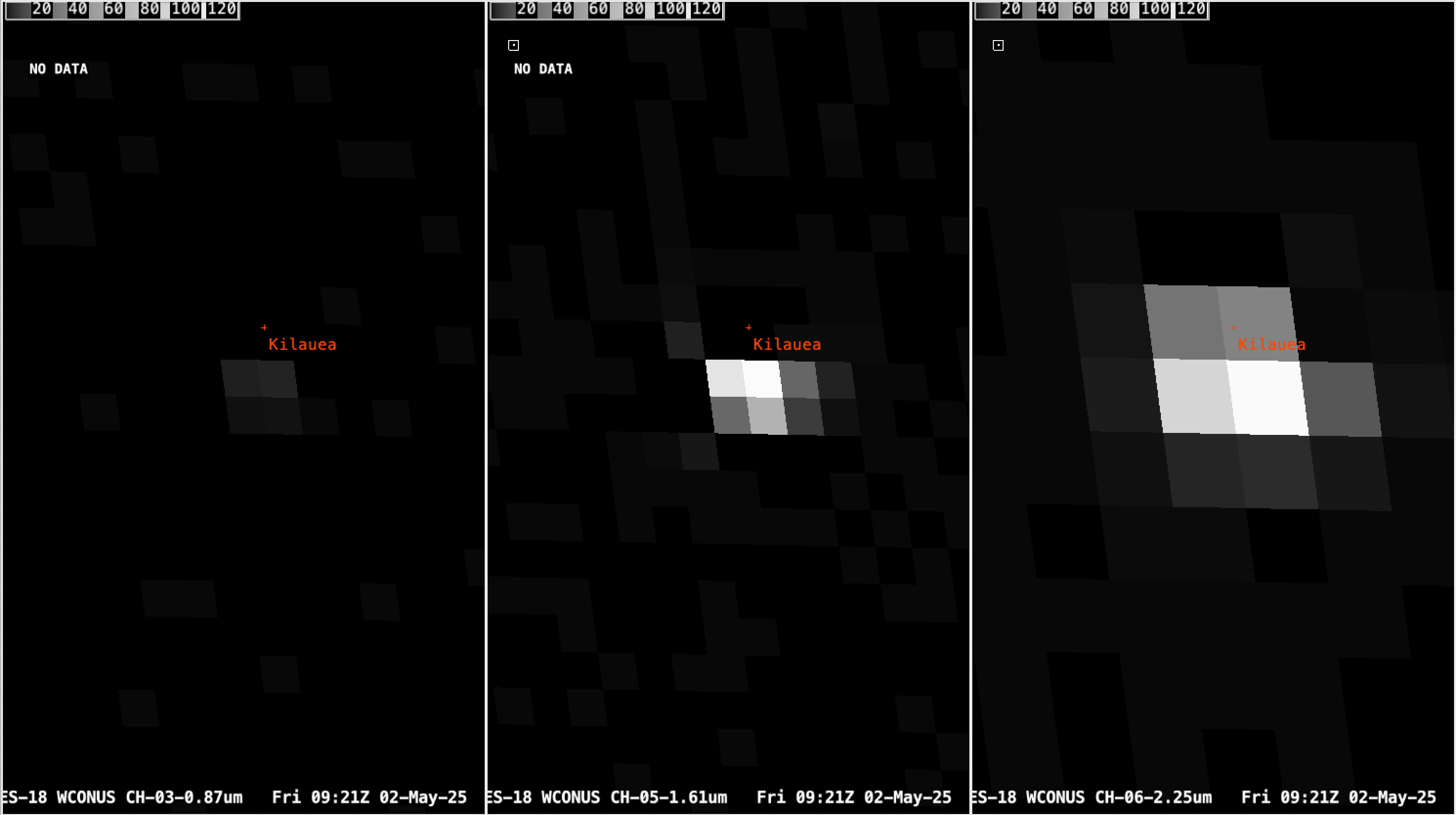
Since this latest episode of the Kilauea eruption began during the nighttime hours, its thermal signature was also apparent in GOES-18 Near-Infrared 0.86 µm, 1.61 µm and 2.24 µm spectral bands (below).

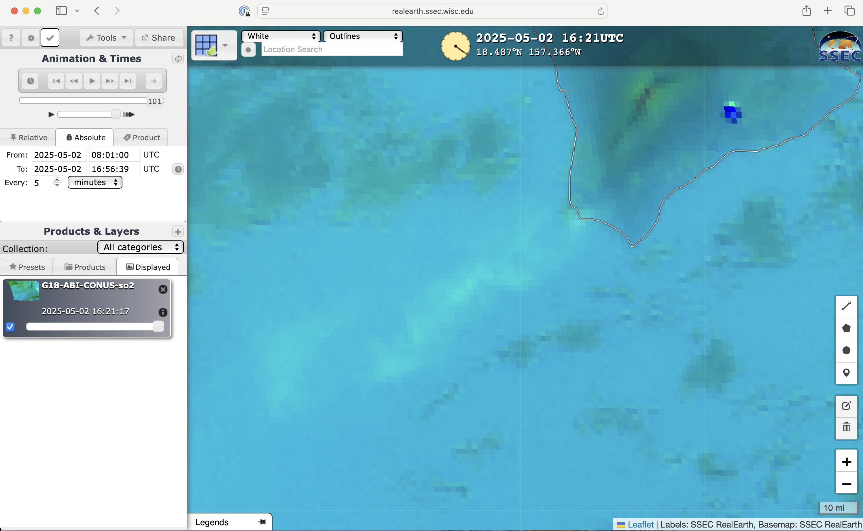
GOES-18 SO2 RGB images from the RealEarth site (below) indicated that a low-altitude plume of SO₂ (pale shades of green) was drifting southwest from Kilauea — the cluster of dark blue pixels denoted the thermal anomaly associated with the eruption site.

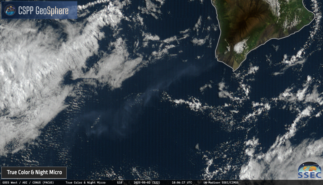
GOES-18 True Color RGB images from the CSPP GeoSphere site (below) showed the southwest transport of hazy volcanic fog (vog) — a mixture of SO₂, CO₂ and water vapor — from the Kilauea eruption site.

View only this post Read Less

When Himawari-10 launches (currently scheduled for late 2028/early 2029), it will carry the GHMS, the Geostationary HiMawari Sounder, planned to give hourly sounder imagery (with more frequent observations — about 4 per hour — in smaller targetable domains, including one over Japan.) The Sounder will observe with about 4-km spatial resolution within two spectral ranges, 4.44 µm – 5.92 µm and 9.13 µm – 14.7 µm. (The information above comes from this presentation). That spectral resolution is similar to the midwave/longwave converage on the CrIS instrument that flies on JPSS Satellites NOAA-20/NOAA-21 and Suomi-NPP. This blog post, the first in a series, shows spectra from CrIS and relates it to the observed atmosphere as a way of preparing National Weather Service staff in the Guam office to use the data. (CrIS data are downloaded in real time at the Direct Broadcast antenna at the Guam Office).

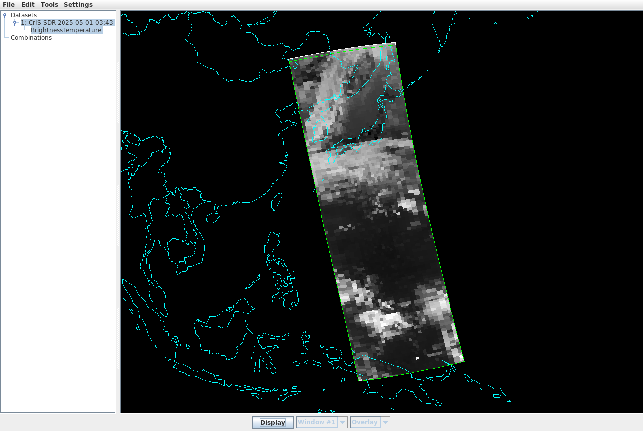
On 1 May 2025, NOAA-20 overflew the Marianas Islands at around 0350 UTC. Following the steps outlined in this blog post, NOAA-20 CrIS data were ordered from the NOAA CLASS site (here’s the list of files; Hydra expects the CrIS data — ‘SCRIF’ — and geolocation data — ‘GCRSO’ — to be combined) and were uploaded into a version of McIDAS-V that can read and interpret CrIS files. The swath loaded is shown below with the Hydra window spawned by McIDAS-V. Note the ‘Display’ button at the bottom of this window.

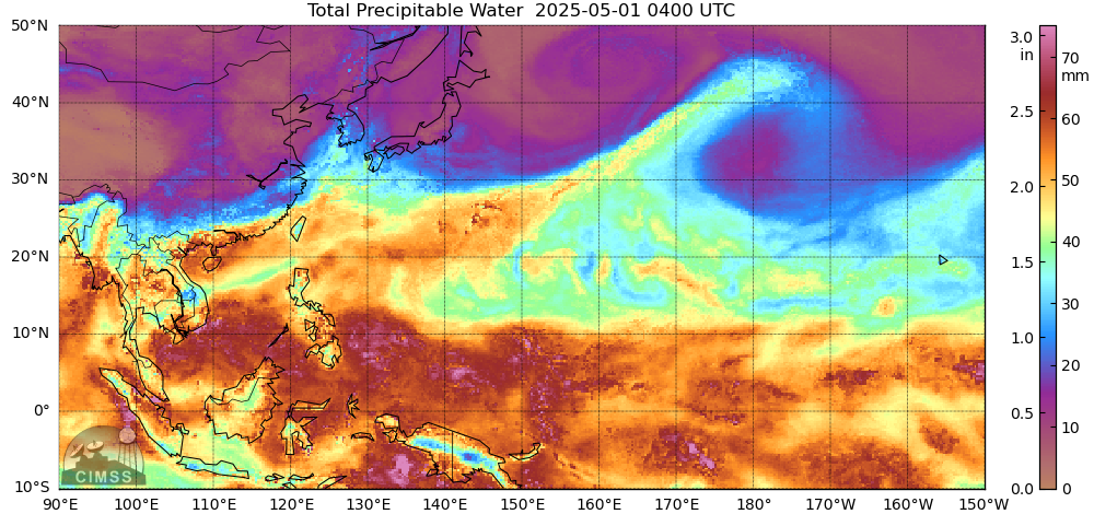
What did other satellite data show over the region? MIMIC Total Precipitable Water (TPW) fields (from this source), below, show relatively dry air around Japan and over the central Pacific between 10^o and 20^oN.

I also used geo2grid software applied to Himawari Standard Data (HSD) files and created the True Color and airmass RGB images below. The relative dryness in a longitudinal strip through Guam is apparent, as are the more moist regions to the north and south.

---

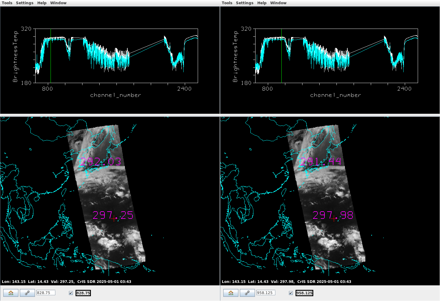
Now that you have a gross understanding of the atmosphere in this region, what do you expect the spectra to look like over this region? Clicking that ‘Display’ button in the McIDAS-V Hydra window spawns an interactive window, two examples of which are shown below. Two spectra are shown: the cyan spectra is derived from data at the northernmost point, showed over Japan; the white spectra is derived from data closer to Guam. The horizontal mapping of data in the images on the bottom in the figures is at the wavenumber that matches the vertical green line, i.e., wavenumber 828.75 (equivalent to 12.07 µm) on the left and 958.125 (equivalent to 10.44 µm) on the right. The wavenumber to wavelength conversion was done here.

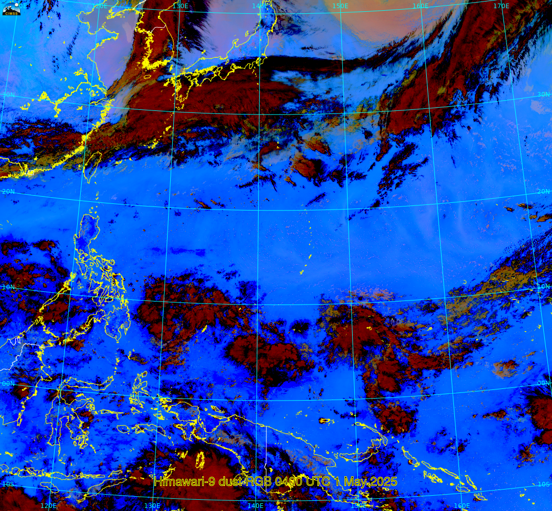
What can you infer from those spectra at the two different points? Note first the strong cooling where ozone absorption is present at wavenumbers around 1050. Wavenumbers exceeding 2200 — the shortwave part of the electromagnetic spectrum — are not slated to be observed by GHMS. Pay attention to the slope of the two spectra between 800 and 1000; in the white line, brightness temperature change more over the range over Guam — the white line — compared to over Japan — the cyan line. Brightness temperature differences plotted at the points on the map over Guam are 297.98 K in the clean window at 10.44 µm and 297.25 K in dirty window at 12.07 µm, for a difference of 0.73 K and over Japan are 291.44 K in the clean window (10.44 µm) and 292.03 (12.07 µm), for a difference of -0.59K! (Editors note: I was not expecting this, and when I saw that, my reaction was to create the dust RGB below) The negative difference suggest the presence of dust and the dust RGB shows a pinkish hue around Japan, a color in that RGB that is consistent with dust. You can infer something about the atmosphere from the slope of the the spectrum between wavenumbers 830 and 960. If it shows increasing temperatures, i.e., warming, then the atmosphere is likely moist. If it shows level or decreasing brightness temperatures, maybe dust is present.

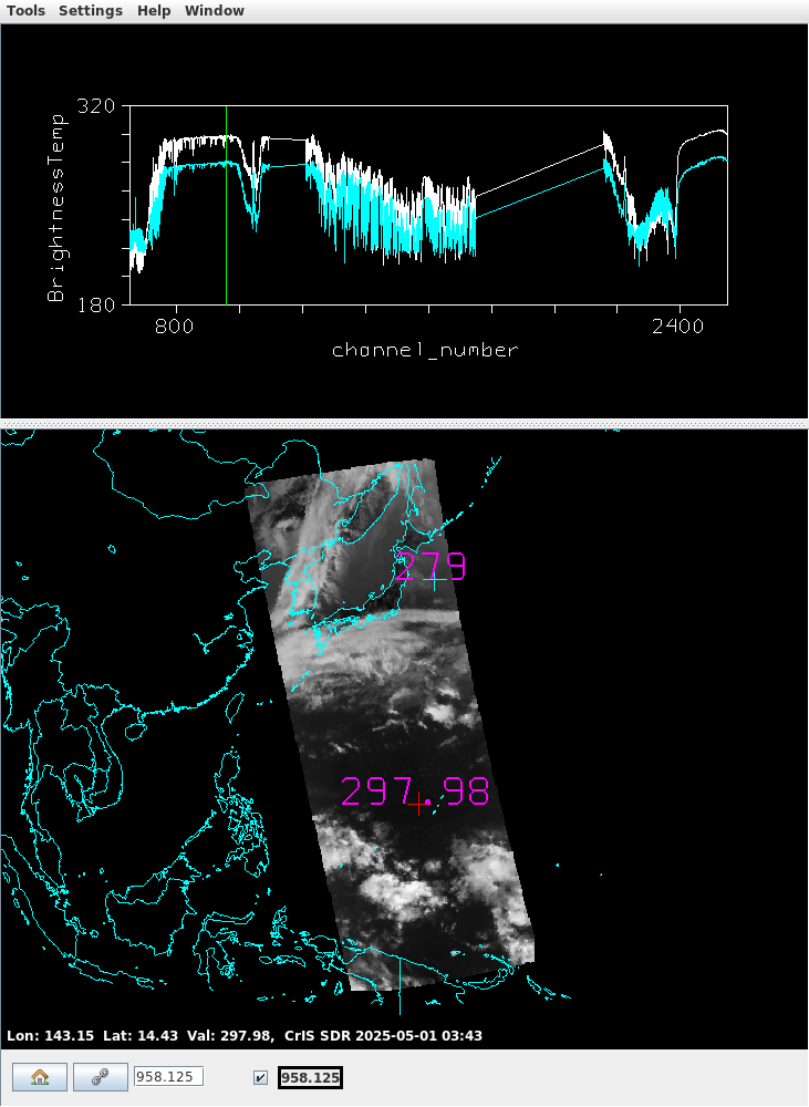
In the spectrum below, the northern point has been moved out of the region where the dust RGB suggests dust is present. The slope of the cyan spectra shows warming brightness temperatures from wavenumbers 800 to 980 is consistent with a decrease of water vapor absorption as observations move from the dirty window to the clean window in the infrared spectrum.

---

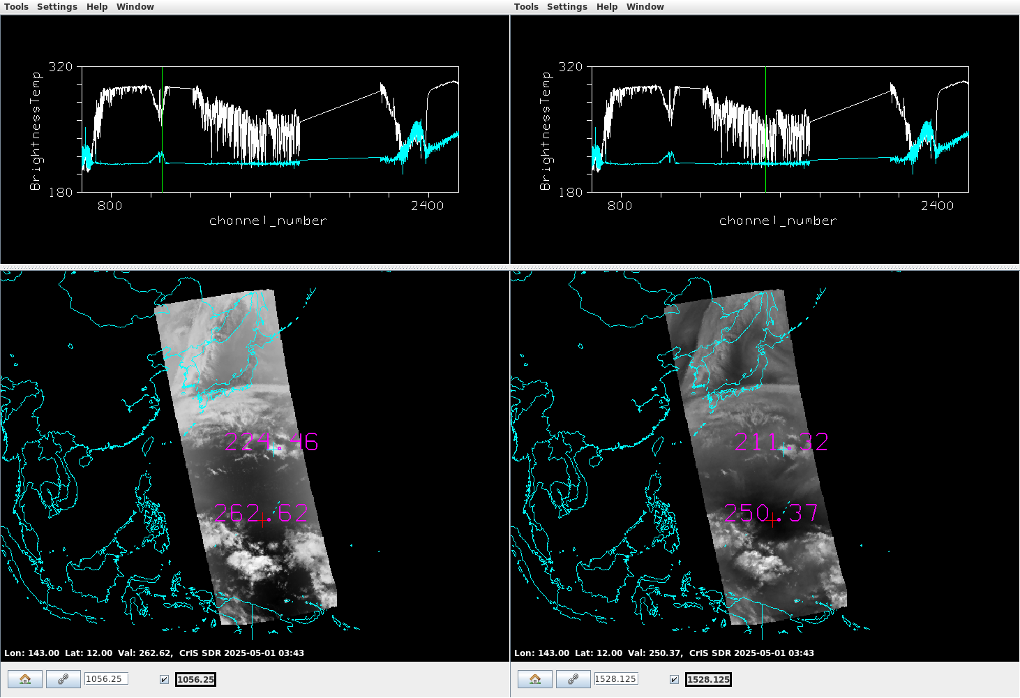
Two different points are examined in the plots below. The greyscale plot on the left is wavenumber 1056.25 (or 9.46 µm, in a region of ozone absorption) and the one of the right is 1528.125 (or 6.5 µm, a region of water vapor absorption). The cyan spectra corresponds to the point centered over convection; the white spectra is in the warmest region at 6.5 µm. The cyan spectrum — a region of cloudiness, as the ‘+’ is centered over a convective cloud — is (mostly) uniformly cold except in the Ozone Absorption band where the spectra shows a local maximum in brightness temperature, and in the shortwave infrared (wavenumbers around 2400 are at 4) where solar radiation is present and in the longwave (wavenumbers around 750 are at 13.3) where CO2 absorption will have an effect. In the white spectrum, at a point in clear air, ozone absorption does not have a warming effect, and the large valley of variable water vapor absorption from wavenumbers 1200-1600 is apparent. In addition, surface features are not discernible at these wavenumbers unlike in the window channels (wavenumbers 828 and 958) shown above.

---

This is the first of several posts on this topic. Stay tuned!

View only this post Read Less