geo2grid (see this recent blog post) is a handy software package that allows anyone to create useful satellite imagery. Recent blog posts that document how to use geo2grid have shown visible or red-green-blue (RGB) composites. Individual infrared bands can also provide useful information, and this blog posts describes how you can create infrared imagery... Read More
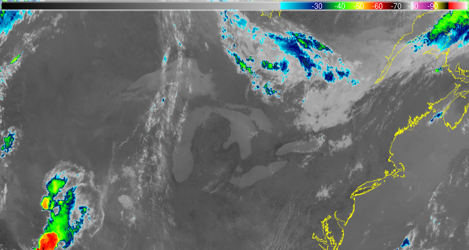
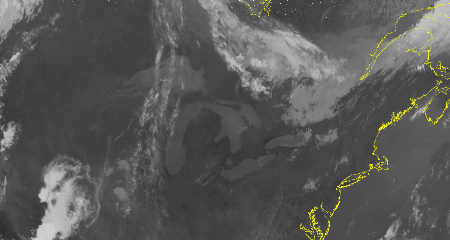
GOES-16 ABI Band 13 (10.3 µm) Infrared Imagery from 1550 UTC on 2 July 2020, with color enhancement added, and with annotated colorbar (Click to enlarge)
geo2grid (see this recent blog post) is a handy software package that allows anyone to create useful satellite imagery. Recent blog posts that document how to use geo2grid have shown visible or red-green-blue (RGB) composites. Individual infrared bands can also provide useful information, and this blog posts describes how you can create infrared imagery to which a useful color enhancement has been applied.
Step 1, as always, is to find data. NOAA CLASS has archived Level-1b Radiance files; these are the data that geo2grid expects, and the naming convention of the files is also what geo2grid expects. Amazon Cloud Services can also offer correctly-named data. (This blogger is aware of some users who have retrieved data from Google, and those files did not follow the expected naming convention).
The animation above compares an infrared image from 1550 UTC on 2 July over the northern part of the United States. The grid is described in this blog post and was used for convenience. (Of some importance: The grid created has dimensions of 1500×800). The original grey-scaled image is shown (with coastlines overlain), then a color enhancement is applied, and finally a script is run to annotate the colorbar.
The geo2grid command used to start the image creation was:
./geo2grid.sh -r abi_l1b -w geotiff -p C13 -g PADERECHO --grid-configs $GEO2GRID_HOME/PADERECHO.conf --method nearest -f /arcdata/goes_restricted/grb/goes16/2020/2020_07_02_184/abi/L1b/RadF/OR_ABI-L1b-RadF-M6C13_G16_s20201841550211_e20201841559531_c20201841600013.nc
This creates a Band 13 (the -p C13 flag) grey-scaled geotiff (-w geotiff) from data at the archive site specified ( -f /arcdata/goes_restricted/..../OR_ABI-L1b-RadF-M6C13_G16_s20201841550211_e20201841559531_c20201841600013.nc ), reading Advanced Baseline Imagery Level-1b imagery (the -r abi_l1b flag), and using nearest-neighbor interpolation to a pre-defined grid (“PADERECHO”) to transform the projection from the default satellite projection (That’s this part of the command: -g PADERECHO --grid-configs $GEO2GRID_HOME/PADERECHO.conf --method nearest). Note that by default, the geotiff created is 8-bit (in contrast to the 11-bit imagery; some information is lost.) You can create geotiffs with full bit depth. For this example an 8-bit image is being created.
The add_colorbar shell applies a color enhancement to the grey-scaled geotiff image that geo2grid creates. For the image in this blog post, I used this invocation:
./add_colormap.sh ../../enhancements/IR4AVHRR100_colortable.txt GOES-16_ABI_RadF_C13_20200702_155021_PADERECHO.tif
This colorbar must be pre-defined by the user. The format of the colortable (“IR4AVHRR100_colortable.txt”) is a comma-separated list of greyscale values (0-255 for the 8-bit geotiff that is created) followed by Red, Green, Blue and Transparency values. (Documentation is here. The file used for this example is here — courtesy of Jim Nelson, CIMSS) The colortable is applied to the geotiff image and a separate image (.png in this case) is created. You will note that this bi-linear enhancement is various shades of grey for bit values 0-152, then different colors for values 153-255.
How do you associate the color with a temperature? For a bi-linear enhancement as used for Band 13, this is not simple. With knowledge of the calibration used, or with access to a system (such as McIDAS-X or McIDAS-V) that includes the calibration, it is possible to associate the greyscale values with temperature values and then use annotation software such as ImageMagick to write in values, with a command such as:
convert INPUTFIELD_with_Coastline_Colorbar_Enhanced.png -fill white -pointsize 24 -annotate +997+28 "-30" InputField_with_CoastLine_Colorbar_enhanced_-30Label.png
This must be done for each label you want to add to the image, but a shell script does this easily, and once done, you have something that you can use for any image that is the same size: 1500 pixels wide. The spacing between the -30ºC, -40ºC, -50ºC… labels on the color bar is constant in this example. Thus, once two values are known and placed, it’s simple to compute the offsets for the other temperature values.
Polar2Grid colorbar functionality is a bit more comprehensive than Geo2Grid. When a colorbar is created in Polar2Grid, metadata on the minimum and maximum values are inserted into the geotiff. This allows automatic generation of colorbar labels (for a linear scaling only) as shown in this excellent example of documentation!
View only this post
Read Less
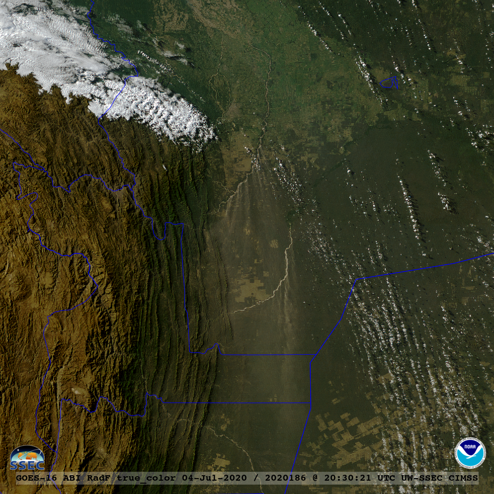
![GOES-16 True Color RGB images [click to play animation | MP4]](https://cimss.ssec.wisc.edu/satellite-blog/images/2020/07/GOES-16__ABI_RadF_true_color_Bolivia_2020186.gif)
![VIIRS True Color RGB images from Suomi NPP and NOAA-20 [click to enlarge]](https://cimss.ssec.wisc.edu/satellite-blog/images/2020/07/200704_suomiNPP_noaa20_viirs_trueColorRGB_blowing_dust_Bolivia_anim.gif)
![Plot of surface report data from Viro Viru International Airport [click to enlarge]](https://cimss.ssec.wisc.edu/satellite-blog/images/2020/07/200704_SLVR_SFCMG.GIF)

