This website works best with a newer web browser such as Chrome, Firefox, Safari or Microsoft
Edge. Internet Explorer is not supported by this website.
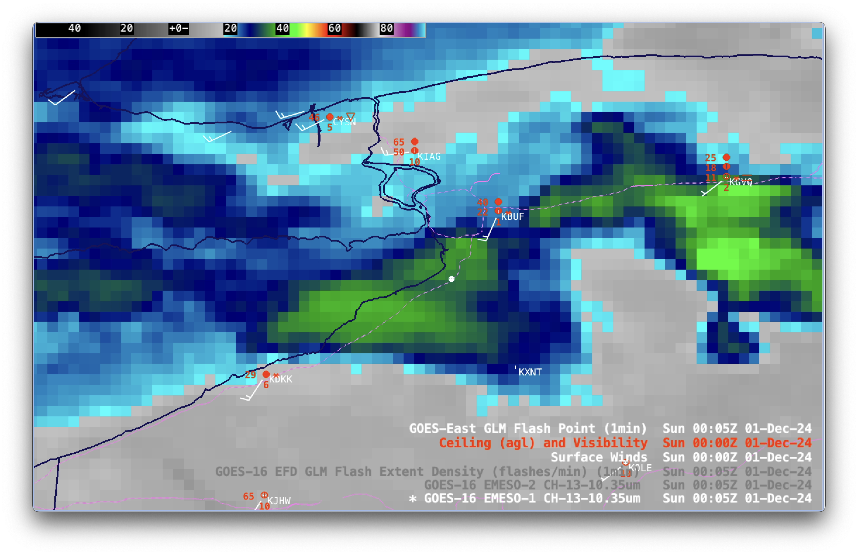
1-minute Mesoscale Domain Sector GOES-16 (GOES-East) Clean Infrared Window (10.3 µm) images (above) showed a lake effect snow (LES) band that intensified over far eastern Lake Erie, shortly before moving inland across western New York after sunset on 30th November 2024. Intermittent lightning activity was seen immediately inland as the LES band moved across... Read More
1-minute GOES-16 Clean Infrared Window (10.3 µm) images, with plots of Ceiling and Visibility (red), wind barbs (white) and GLM Flash Points (white dots), from 2300 UTC on 30th November to 0400 UTC on 1st December; Interstate Highways are plotted in magenta [click to play MP4 animation]
1-minute Mesoscale Domain Sector GOES-16 (GOES-East) Clean Infrared Window (10.3 µm) images (above) showed a lake effect snow (LES) band that intensified over far eastern Lake Erie, shortly before moving inland across western New York after sunset on 30th November 2024. Intermittent lightning activity was seen immediately inland as the LES band moved across Interstate 90 between Buffalo (KBUF) and Dunkirk (KDKK), with several GLM Flash Points appearing.
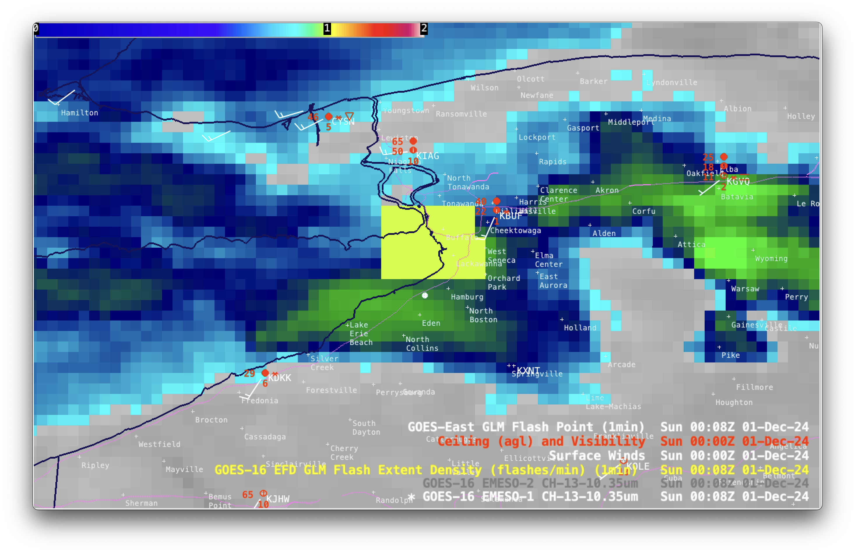
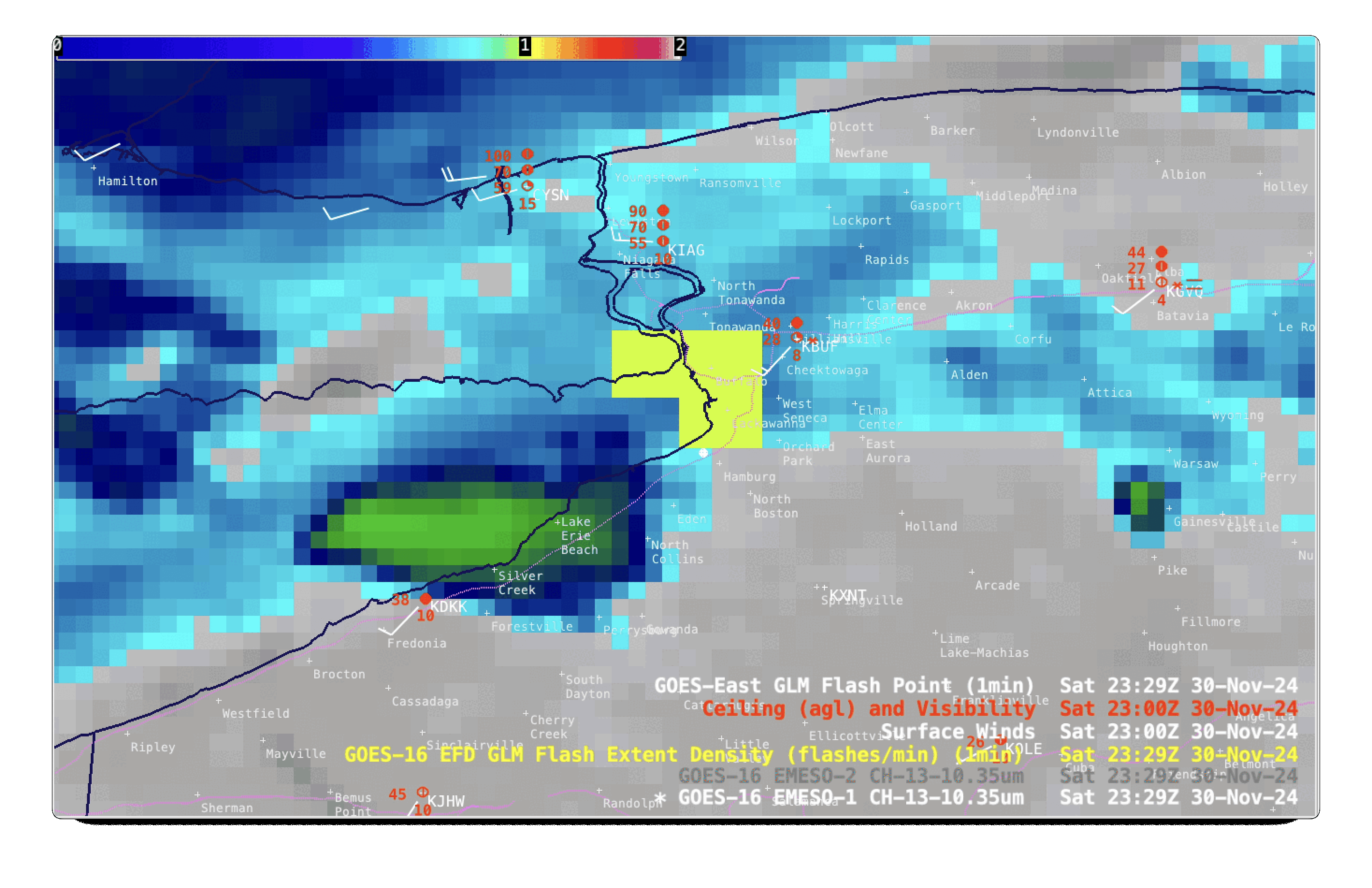
A similar animation of GOES-16 Infrared images included overlays of both GLM Flash Extent Density and Flash Points (below). Note the slight northward displacement of the Flash Extent Density pixels compared to the Flash Points — this is because commonly-used Gridded GLM products (such as Flash Extent Density, Minimum Flash Area and Total Optical Energy) are not corrected for parallax, as the GLM Flash Points are.
1-minute GOES-16 Clean Infrared Window (10.3 µm) images, with plots of Ceiling and Visibility (red), wind barbs (white), GLM Flash Extent Density (large yellow to white pixels) and GLM Flash Points (white dots), from 2300 UTC on 30th November to 0400 UTC on 1st December; Interstate Highways are plotted in magenta [click to play MP4 animation]
A stepped sequence of 6 times with GLM observations (2329 UTC/2339 UTC/2345 UTC/0005 UTC/0008 UTC/0051 UTC) is shown below, to provide an easier examination of the displacement between GLM Flash Extent Density and GLM Flash Points. Much of this satellite-detected lightning activity was occurring near Lackawanna (south of Buffalo), where thundersnow was observed.
GOES-16 Clean Infrared Window (10.3 µm) images, with plots of Ceiling and Visibility (red), wind barbs (white), GLM Flash Extent Density (large yellow to white pixels) and GLM Flash Points (white dots); Interstate Highways are plotted in magenta [click to enlarge]
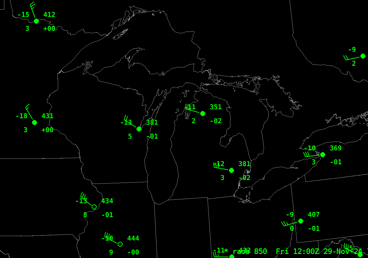
Cold air over the Great Lakes (see the plot of 850-mb temperature from RAOB stations at 1200 UTC below; note the similarity in temperatures and wind speeds over the Great Lakes states) means Lake Effect Snow. The animation above (source) shows snow bands over western lower Michigan and also downwind... Read More
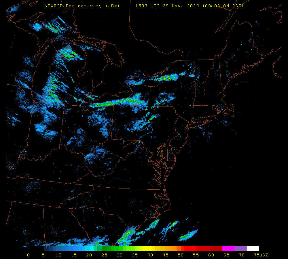
NEXRAD relfectivity over the northeastern US and Great Lakes, 1503-1813 UTC on 29 November 2024 (Click to enlarge)
Cold air over the Great Lakes (see the plot of 850-mb temperature from RAOB stations at 1200 UTC below; note the similarity in temperatures and wind speeds over the Great Lakes states) means Lake Effect Snow. The animation above (source) shows snow bands over western lower Michigan and also downwind of Lake St. Clair, and in a single band over Lake Erie. An interesting aspect to this animation (to your blogger, at least), is the distance before the radar detection of snow occurs is pretty large over Lake Michigan, but the band development is almost immediate over Lake St. Clair and just a bit slower over Lake Erie. In addition, lake-effect band development over Lake Ontario is a bit slower than over Erie. Why?
RAOB plots, 1200 UTC on 29 November 2024 (Click to enlarge)
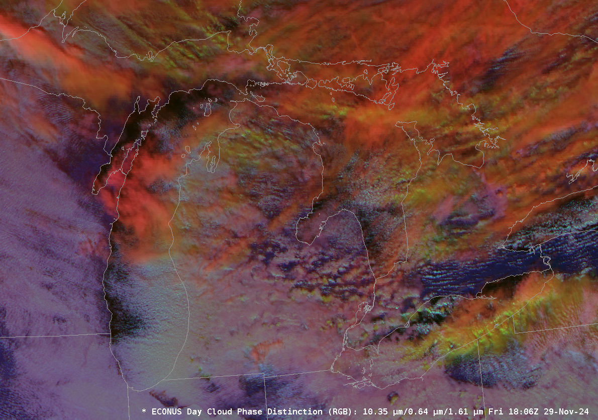
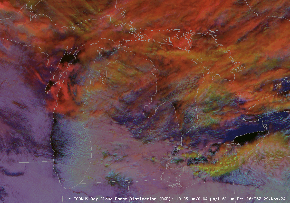
Day Cloud Phase Distinction RGB Imagery from near Noon, below, shows that the bands over Lakes Erie and St. Clair are likely glaciating almost immediately (this is based on the color — yellowish/green — of the RGB in those bands) compared to non-glaciated clouds (cyan or reddish in the RGB) over western Michigan with the lake-effect there. The atmospheric motions one might infer from the cloud and radar motions is from Lake Michigan (where moisture is added to the lower troposphere) across southern Michigan. Once the air re-emerges over Lake Erie, the moisture added over Lake Michigan means an atmosphere more pre-conditioned to the development of clouds.
GOES-16 Day Cloud Phase Distinction RGB, 1636-1806 UTC on 29 November 2024 (Click to enlarge)
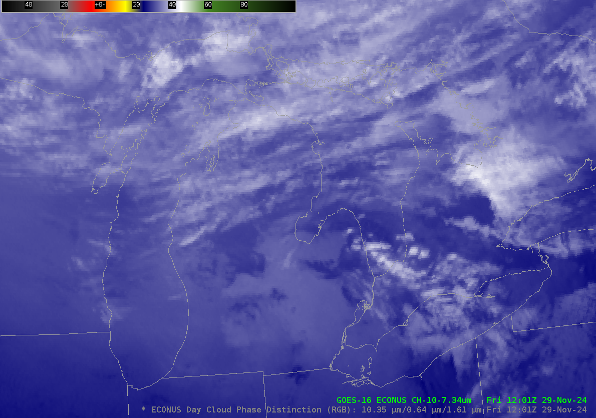
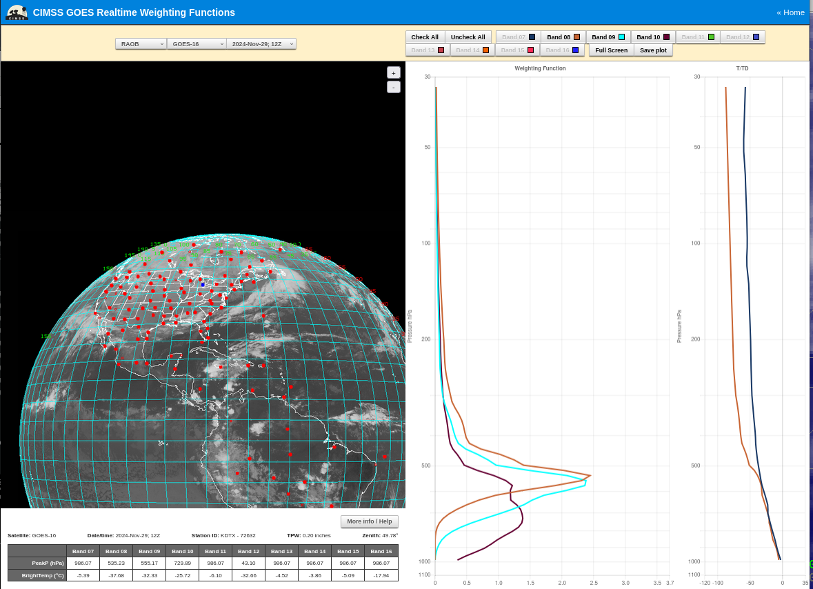
GOES-East Low-level water vapor infrared imagery, below, at 1200 UTC, shows little variability in that field. This suggests that moisture being added to the atmosphere is confined to the lowest part of the atmosphere, below what is detected by the 7.3 µm band. The weighting function for KDTX (that is, White Lake Michigan near Detroit), below, shows information at 7.3 µm is predominantly from the 600-700 mb (assuming clear skies, an admittedly dubious assumption). The GeoXO (the follow-on to the GOES-R series of satellites, scheduled to launch in the mid-2030s) satellite will detect radiation at 5.15 µm, a wavelength that allows moisture detection at even lower levels than bands on GOES-16/GOES-18; perhaps that channel will detect the moistening caused by Lake Michigan that allows Lake Effect Bands to develop more rapidly over downwind lakes, given a suitable trajectory.
GOES-16 Low-Level water vapor infrared imagery (Band 10, 7.3 µm) at 1201 UTC on 29 November 2024 (Click to enlarge)Weighting Functions for Bands 8,9,10 at KDTX, 1200 UTC 29 November 2024 (Click to enlarge)
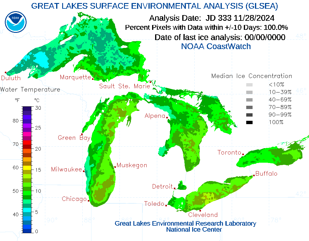
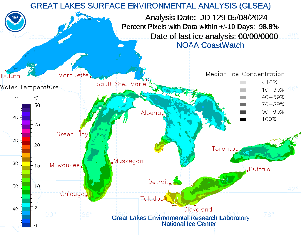
For those (correctly!) wondering if lake surface temperatures might drive the difference in band development, consider the temperature analysis below for 28 November 2024 (source). Michigan and Erie temperatures are very similar.
Great Lakes Surface Temperature Analysis valid 28 November 2024 (Click to enlarge)
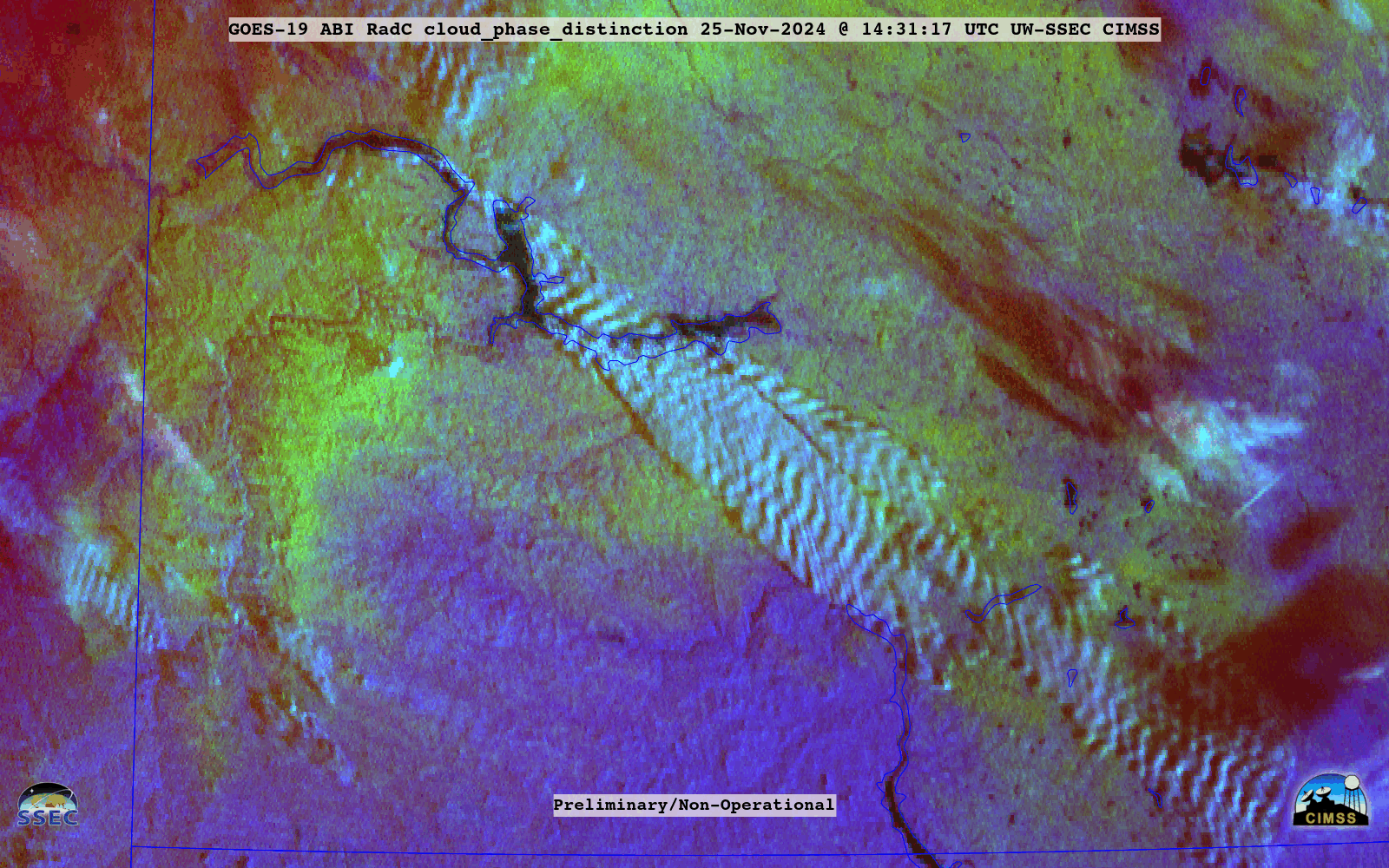
GOES-19 (Preliminary/Non-operational) Day Cloud Phase Distinction RGB images (above) — created using Geo2Grid — displayed supercooled “lake effect” clouds (shades of white) streaming southeast off Lake Sakakawea in northwestern North Dakota on 25th November 2024. A smaller cloud plume was also seen streaming southeast off Devils Lake in northeastern North Dakota. Existing snow cover appeared as shades of green... Read More
GOES-19 (Preliminary/Non-operational) Day Cloud Phase Distinction RGB images, from 1431-2216 UTC on 25th November [click to play animated GIF | MP4]
GOES-19 (Preliminary/Non-operational) Day Cloud Phase Distinction RGB images (above) — created using Geo2Grid — displayed supercooled “lake effect” clouds (shades of white) streaming southeast off Lake Sakakawea in northwestern North Dakota on 25th November 2024. A smaller cloud plume was also seen streaming southeast off Devils Lake in northeastern North Dakota. Existing snow cover appeared as shades of green in the RGB images, with bare ground appearing as shades of blue.
GOES-16 (GOES-East) Near-Infrared “Snow/Ice” (1.61 µm) images (below) included 15-minute plots of METAR surface reports — which showed brief periods of light snow at Hazen (KHZE) and Bismarck (KBIS). Snow cover appeared as darker shades of gray to black in the Snow/Ice imagery. Note the cold air — having temperatures in the single digits to teens F — that was flowing across the still-unfrozen reservoirs of the Missouri River (in addition to Devils Lake). Water surface temperatures on Lake Sakakawea were in the middle to upper 40s F.
GOES-16 Near-Infrared “Snow/Ice” (1.61 µm) images, with 15-minute METAR surface reports plotted in cyan, from 1416-2231 UTC on 25th November [click to play animated GIF | MP4]
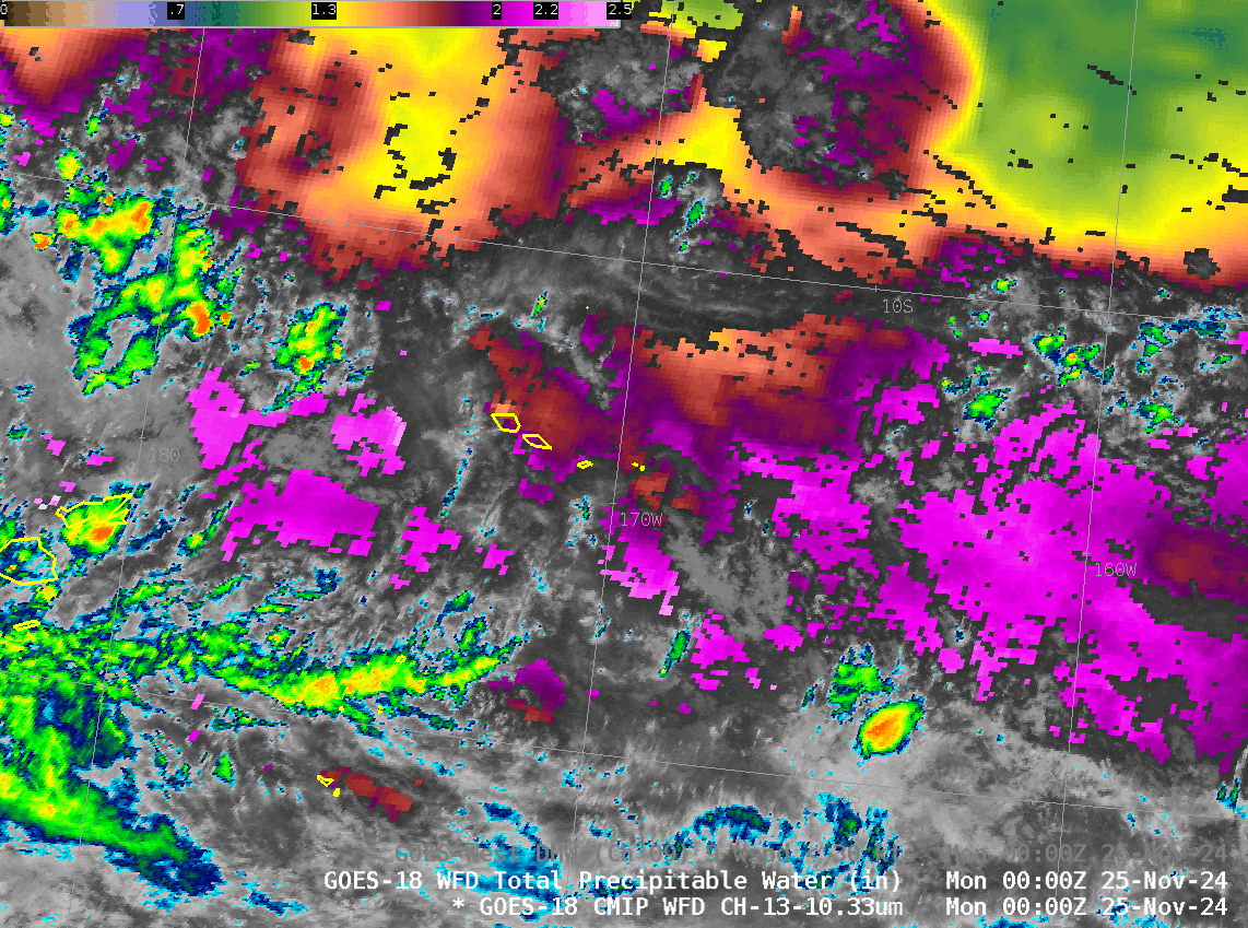
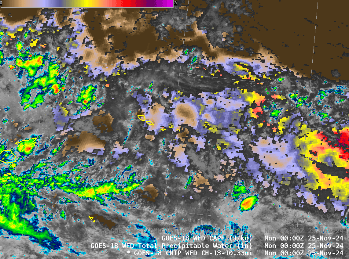
GOES-West imagery centered over the Samoan Islands, shown above in an animation, shows a region of rich moisture surrounding those islands (purple in the enhancement, which suggests values or 2-2.2″), but the islands themselves are within a dry pocket (TPW values closer to 1.7″, orange/rust in the enhancement used). Total... Read More
GOES-18 Band 13 Clean Window infrared (10.3 µm) imagery and clear-sky estimates of Total Precipitable Water, 0000 – 1531 UTC on 25 November 2024 (Click to enlarge)
GOES-West imagery centered over the Samoan Islands, shown above in an animation, shows a region of rich moisture surrounding those islands (purple in the enhancement, which suggests values or 2-2.2″), but the islands themselves are within a dry pocket (TPW values closer to 1.7″, orange/rust in the enhancement used). Total Precipitable Water derived from Microwave data, below (from the MIMIC website), shows similar values, including the local minimum over Samoa. A benefit with microwave observations of atmospheric moisture (compared to ABI) is the ability to detect values in the presence of clouds.
MIMIC Total Precipitable Water estimates, 1600 UTC 24 November – 1500 UTC 25 November 2024 (Click to enlarge)
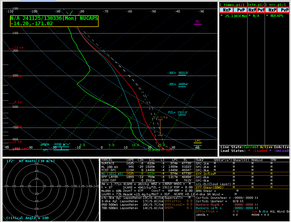
Pago Pago airport does have an upper-air station. However, hydrogen generation difficulties at that site in the past months have meant that balloon launches are limited, and one did not occur at 1200 UTC on 25 November. However, NOAA-20 overflew the region shortly thereafter and NUCAPS soundings can estimate the thermodynamic profile. The plot below shows where profiles are available; green points signify profiles for which the infrared retrieval converged to a solution, typically in regions of mostly clear skies (as might be inferred from the GOES-18 imagery above!)
NUCAPS Sounding Availability plots in the south Pacific Ocean, ca. 1230 UTC on 25 November 2024 (Click to enlarge)
The toggle below shows two NUCAPS profiles, one just west of Tutuila (at 14.2oS, 171.5oW) and one 6 points to the south (at 16.55oS, 171.5oW). Note the larger values of TPW in the more southerly sounding, consistent with what is discussed above. Otherwise, the profiles are quite similar.
NUCAPS Profiles near 171.5 W, near Tutuila (at 14.2 S) and south of Tutuila (at 16.55 S), ca. 1304 UTC on 25 November 2024 (Click to enlarge)
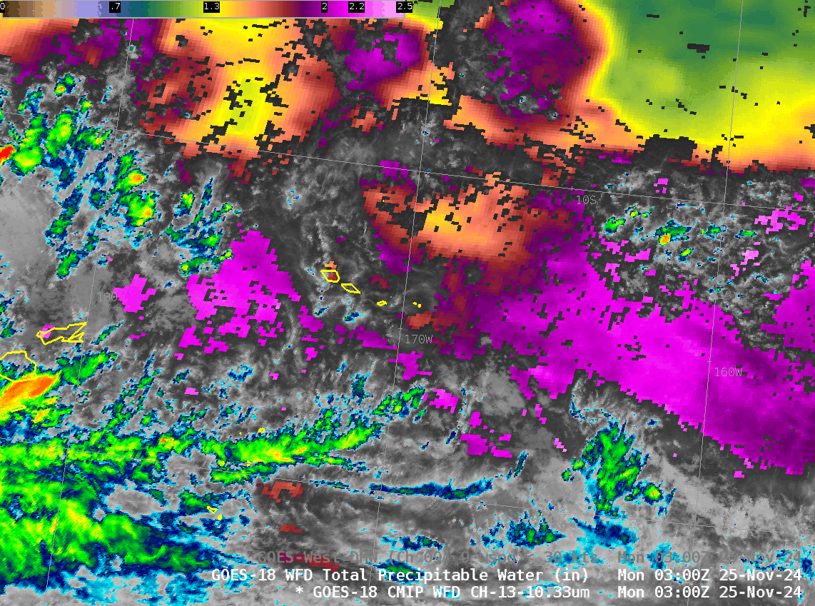
Level 2 products also include clear-sky measures of instability, such as Lifted Index and Convective Available Potential Energy (CAPE). The Lifted Index field below shows pockets of stability (blue in the enhancement used) surrounded by minor instability (yellow in the enhancement) surrounding the Samoan Islands.
CAPE values (scaled from 0-400 J/kg) similarly show relatively weak regions of stability and instability surrounding the Samoan islands.
GOES-West Clean Window infrared (Band 13, 10.3 µm) imagery and clear-sky estimates of CAPE (Scaled from 0-400), 0000 – 1530 UTC On 25 November 2024 (Click to enlarge)
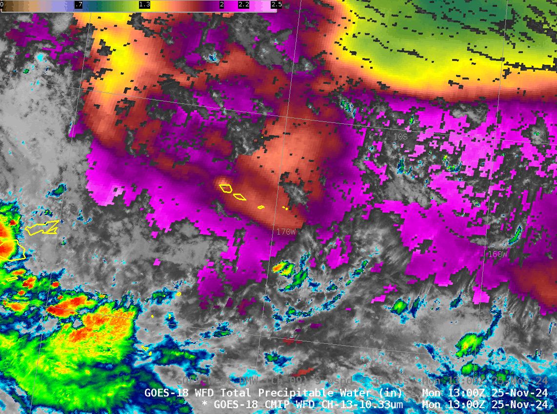
The TPW fields, and the Derived Stability Indices, do have similarities as might be expected. The toggles below compare TPW, LI an CAPE at 0300 and at 1300. Interestingly, the strong values of CAPE at the eastern edge of the domain at 0300 UTC seemingly have no echo in the other fields. In other regions (north of the Samoan Islands, for example), minima in CAPE and relative stability in Lifted Index occur where local minima in TPW exist. This case demonstrates how one stability index might not give the same information as another; make sure you have access to both!
GOES-18 clean window infrared (Band 13, 10.3 µm) imagery under clear sky estimates of Total Precipitable Water, CAPE and Lifted Index, 0300 UTC on 25 November 2024 (Click to enlarge)GOES-18 clean window infrared (Band 13, 10.3 µm) imagery under clear sky estimates of Total Precipitable Water, CAPE and Lifted Index, 1300 UTC on 25 November 2024 (Click to enlarge)
The (anti-clockwise) motion of the cloud features above suggests that an anticylone is present over the islands The animation below includes GOES-West derived motion wind vectors computed from Band 9 (mid-level water vapor, 6.95 µm) infrared images. The wind vectors are from near 350 mb, which height is determined by matching the Band 9 brightness temperature to GFS model temperatures.
GOES-18 clean window infrared (Band 13, 10.3 µm) imagery under clear sky estimates of Total Precipitable Water, with Derived Motion Wind vectors computed with Band 9 (mid-level water vapor) infrared imagery, 0000-1530 UTC on 25 November (Click to enlarge)
Level 2 Products, especially in regions — like the South Pacific Ocean — where conventional data are lacking, can give a forecaster needed insight into how the atmosphere might evolve with time.


