GOES-16 ABI Band 13 (10.3 µm) infrared imagery, 1901 6 June 2020 – 0656 7 June 2020 (Click to play mp4 animation)
Several satellite-based thermodynamic estimates keyed in on South Dakota as a region where instability was noteworthy. The GOES-16 All-Sky Convective Available Potential Energy (available here), shown below from 2026 UTC on 6 June when values were greatest, for example, showed a persistent corridor of instability across South Dakota.

GOES-16 ‘All-Sky’ estimates of Convective Available Potential Energy, 2026 UTC on 6 June 2020 (Click to enlarge)
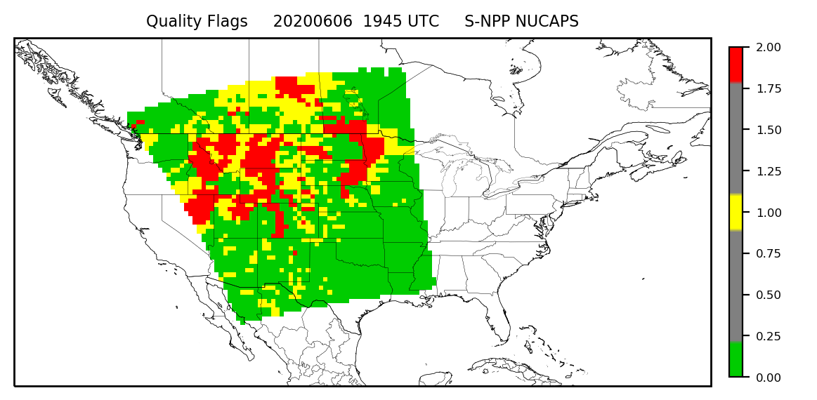
NUCAPS estimates of 700-500 mb lapse rates, below (from this site), show pronounced instability upstream of South Dakota at 1945 UTC, when Suomi-NPP overflew the region. (Most of the soundings used to produce the lapse rate information were from successful infrared retrievals as shown in this graphic).

700-500 mb Lapse Rates derived from Suomi NPP NUCAPS soundings, 1945 UTC on 6 June 2020 (Click to enlarge)
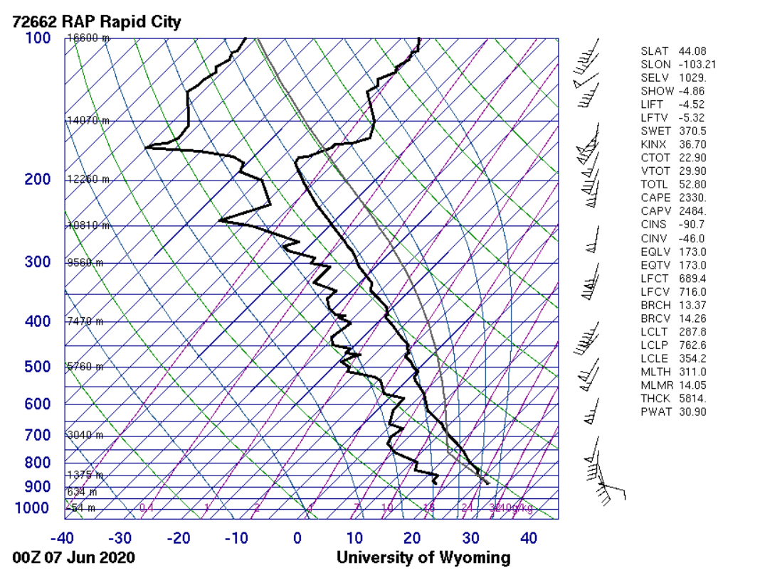
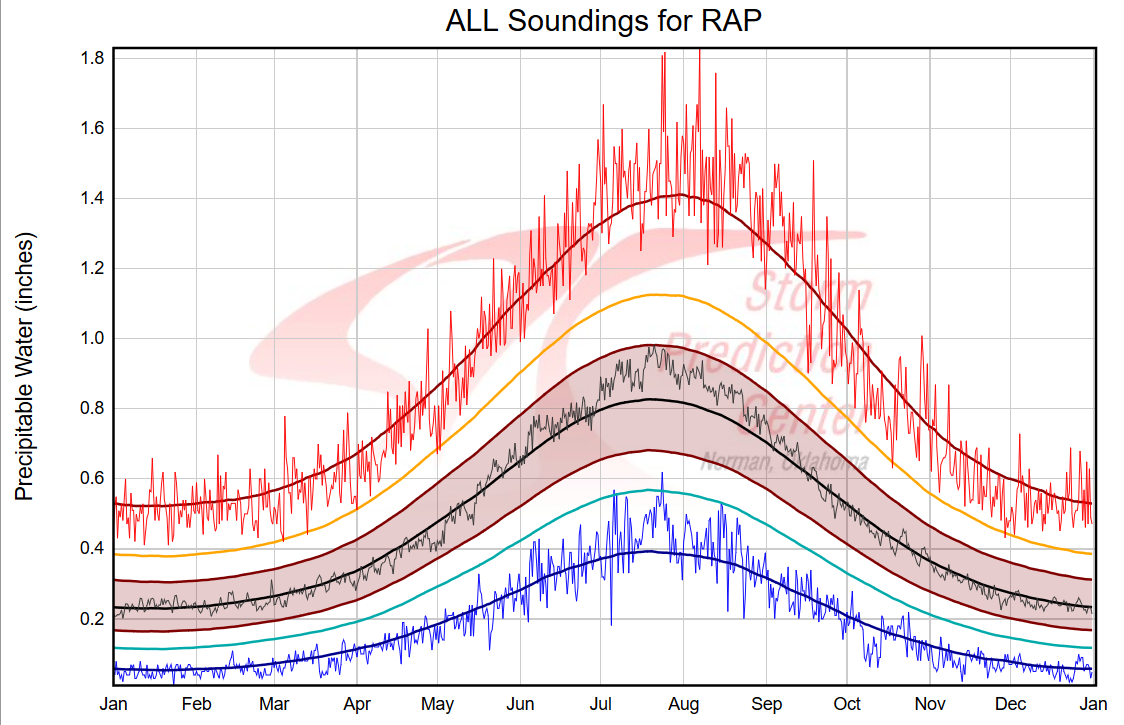
Surface moisture had pooled over western South Dakota. That is shown in the plot below of surface dewpoints showing very unusual (for South Dakota) mid-60s dewpoints! Further evidence of the unusual moisture amounts over the high Plains (for early June) is in this sounding from Rapid City at 0000 UTC on 7 June (source); Precipitable Water is at 1.2″! This value is unusual for the location and time of year, as shown here (Source).
Surface Dewpoints, 2100 UTC on 6 June 2020 over South Dakota and surrounding states (Click to enlarge)
GOES-17 Full-Disk imagery (at 10-minute time-steps) captured an oblique view of the developing convection. (The ‘PACUS’ sector with 5-minute imagery terminates in west-central South Dakota so is not used here; A GOES-17 Mesoscale sector was not in place for this event, although a GOES-16 one was).
GOES-17 Visible Imagery (0.64 µm) on 7 June 2020, 0000 – 0220 UTC (Click to animate)
1-minute Mesoscale Domain Sector GOES-16 “Red” Visible images with time-matched plots of SPC Storm Reports are shown below.
![GOES-16 “Red” Visible (0.64 µm) images [click to play animation | MP4]](https://cimss.ssec.wisc.edu/satellite-blog/images/2020/06/200606_goes16_visible_spcStormReports_Rockies_Plains_derecho_anim.gif)
GOES-16 “Red” Visible (0.64 µm) images [click to play animation | MP4]
View only this post Read Less
![GOES-16 “Clean” Infrared Window (10.35 µm) images (credit: Pete Porandt, AOS) [click to play MP4 animation]](https://cimss.ssec.wisc.edu/satellite-blog/images/2020/06/200604_0556utc_goes16_infrared_mcs_merger.png)
![GOES-16 “Clean” Infrared Window (10.35 µm) images, with SPC storm reports plotted in cyan [click to play animation | MP4]](https://cimss.ssec.wisc.edu/satellite-blog/images/2020/06/200604_goes16_infrared_spcStormReports_MO_mcs_merger_anim.gif)
![Suomi NPP VIIRS Day/Night Band (0.7 µm) image [click to enlarge]](https://cimss.ssec.wisc.edu/satellite-blog/images/2020/06/mcs_merger_viirs_dnb-20200604_071607.png)
![GOES-16 “Red” Visible (0.64 µm) images [click to play animation | MP4]](https://cimss.ssec.wisc.edu/satellite-blog/images/2020/06/200604_goes16_visible_MO_IL_mcv_anim.gif)
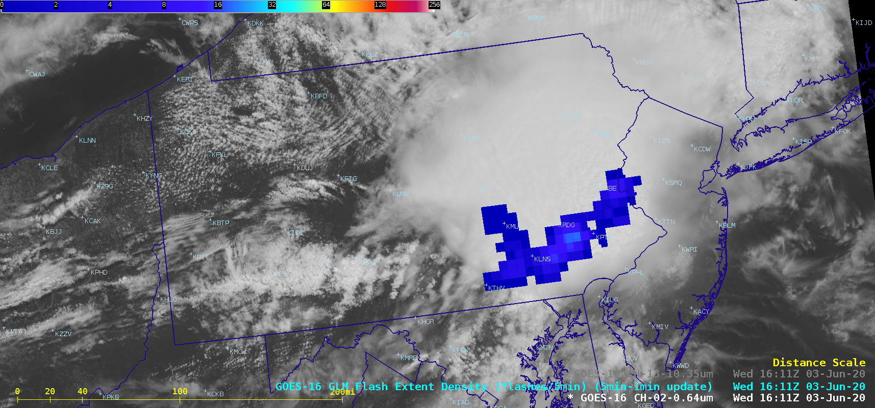
![GOES-16 “Red” Visible (0.64 µm) images, with SPC Storm Reports plotted in red [click to play animation | MP4]](https://cimss.ssec.wisc.edu/satellite-blog/images/2020/06/200603_goes16_visible_spcStormReports_PA_NJ_derecho_anim.gif)

