
10-minute Full Disk scan GOES-18 (GOES-West) daytime True Color RGB and nighttime Dust RGB images created by Geo2Grid (above) highlighted plumes of glacial silt being transported offshore by strong katabatic winds that were occurring in the northern Alaska panhandle on 09-10 December 2025. Note the strong pressure gradient between a ridge of... Read More

10-minute GOES-18 daytime True Color RGB and nighttime Dust RGB images, from 1930 UTC on 09 December to 1200 UTC on 10 December [click to play MP4 animation]
10-minute Full Disk scan GOES-18
(GOES-West) daytime True Color RGB and nighttime
Dust RGB images created by
Geo2Grid (above) highlighted plumes of glacial silt being transported offshore by strong katabatic winds that were occurring in the northern Alaska panhandle on 09-10 December 2025. Note the strong pressure gradient between a ridge of high pressure centered inland over Yukon and a consolidating Gale Force Low over the eastern Gulf of Alaska (
surface analyses).
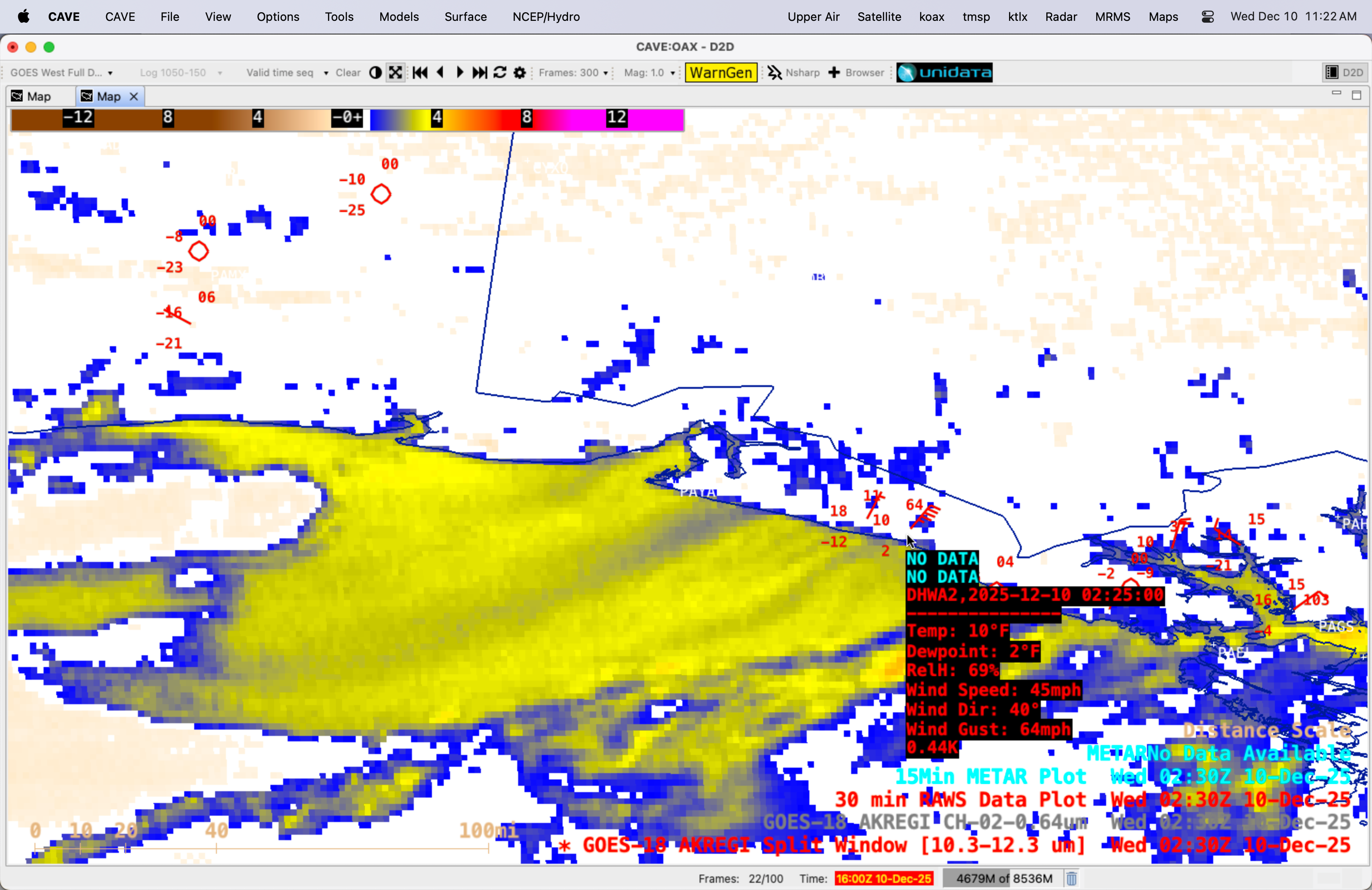
GOES-18 Visible images (below) included plots of METAR and RAWS surface reports — which showed that surface air temperatures at high-elevation inland sites were in the -40s F, compared to around +20 F along the coast. The aforementioned pressure gradient between the cold/dense air inland and the warmer/less-dense air near the coast acted to channel winds through valleys and mountain passes (topography), with these winds accelerating as they approached the coast. During the daytime hours, RAWS site DHWA2 (located 62 miles southeast of Yakutat, PAYA) reported a wind gust to 56 mph at 2225 UTC on 09 December — and after sunset, a wind gust to 64 mph at 0225 UTC on 10 December.

10-minute GOES-18 Visible images, with plots of METAR (cyan) and RAWS (yellow) surface reports, from 1900-2230 UTC on 09 December [click to play MP4 animation]
A NOAA-21 VIIRS True Color RGB image visualized using
RealEarth (below) provided a high-contrast, high-resolution view of the glacial silt plumes as they emerged from the Alaska panhandle coast.

NOAA-21 VIIRS True Color RGB image valid at 2047 UTC on 09 December [click to enlarge]
During the following nighttime hours, there was enough illumination from the Moon — which was in its Waning Gibbous phase, at 72% of Full — to provide a faint signature of the glacial silt plumes in a NOAA-21 VIIRS Day/Night Band image
(below), as changing winds began to transport them southward (a trend that was also seen in nighttime GOES-18
Dust RGB imagery).

NOAA-21 VIIRS Day/Night Band image valid at 1217 UTC on 10 December [click to enlarge]
Metop-B Ultra High Resolution ASCAT winds
(below) showed the narrow plume of katabatic winds emerging from the coast just southeast of Yakutat (at 59.5 N latitude, 139.5 W longitude) at 0448 UTC on 10 December. The broader area of stronger offshore winds farther to the southeast was masked by cloud cover.

Metop-B Ultra High Resolution ASCAT winds at 0448 UTC on 10 December
Similar events involving the offshore transport of glacial silt occur from the Copper River Valley in south-central Alaska.
View only this post
Read Less


