Surface Cold Front over the High Plains of Texas

Hourly GOES-16 ABI Low-Level Water Vapor Infrared (7.34 µm) Imagery, and hourly observations, 0700-1600 UTC on 3 April 2018 (Click to enlarge)
A cold front moving southward along the western Great Plains showed a distinct signature in GOES-16 Water Vapor Imagery. The hourly animation above, with surface observations, shows the front in the Low-Level Water Vapor passing over stations where winds shift from westerly and southwesterly to strong northerly. The feature is far more trackable in GOES-16 ABI Imagery with a 5-minute cadence as is typical over CONUS, as shown below for both low-level water vapor infrared imagery (Band 10, 7.34 µm) and upper-level water vapor infrared imagery (Band 8, 6.19 µm). The infrared imagery allowed a precise determination of when the cold front would reach a location. (In fact, because a GOES-16 Mesoscale Sector was placed over west Texas, the time of arrival could be observed down to the minute, as shown in this animation of the clean window (10.3 µm) infrared imagery from GOES-16).
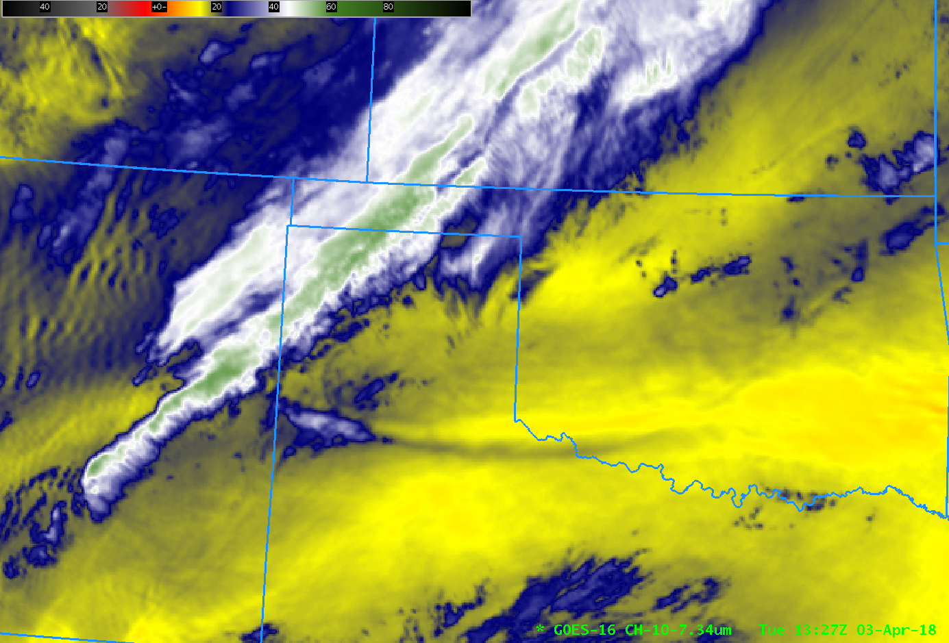
GOES-16 ABI Low-Level Water Vapor Infrared Imagery (7.34 µm), 0832-1637 UTC on 3 April 2018 (Click to animate)
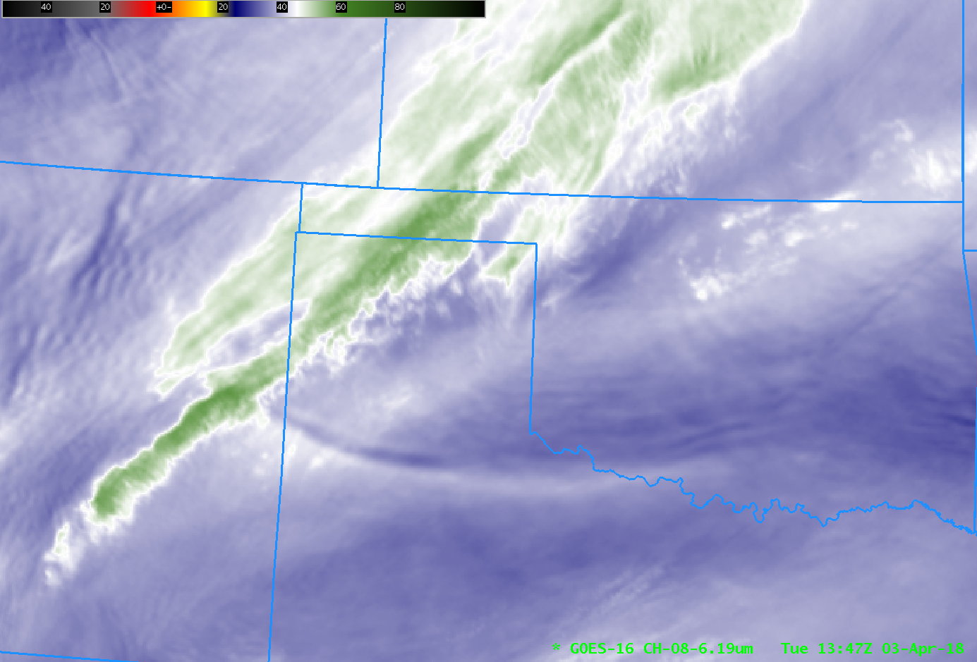
GOES-16 ABI Upper-Level Water Vapor Infrared Imagery (6.19 µm), 0832-1637 UTC on 3 April 2018 (Click to animate)
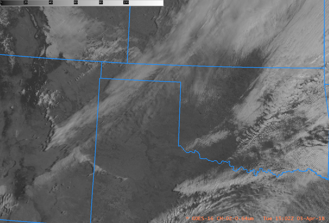
Visible Imagery after sunrise (below) shows that some surface cloudiness was associated with this feature — but other parts were clear.
It is not common for surface features to appear in the Upper-Level Water Vapor Imagery, even when the surface is near 900 mb, as over the High Plains of west Texas. Weighting Functions show from which layers in the atmosphere energy detected by the satellite originates. The Weighting function from Amarillo TX at 1200 UTC on 3 April is shown below. The low-level water vapor weighting function — shown in magenta — shows contributions from the surface, but the upper-level water vapor weighting function — shown in green, shows contributions ending about 200 mb above the surface, at around 700 mb. A conclusion might be that the depth of the cold air quickly increases to around 200 mb behind the front. Thus is can appear in the Upper-Level water vapor imagery. The cold front passes Amarillo (here is a meteorogram) shortly before 1200 UTC (and before the Radiosonde was launched). The radiosonde from Dodge City Kansas, however, at 1200 UTC, shows a cold layer about 200 mb thick. (Here is the Amarillo Sounding for the same time; it’s shown in the Weighting Function plot below as well).
Interpretation of water vapor imagery is simplified if you use information from weighting functions to understand the three-dimensional aspect of the water vapor imagery.
