Plate Tectonics is based on the theory of continental drift proposed by Alfred Wegener in the early 1900’s. Wegener, as well as some before him, recognized the fit of the various continental margins, most notably the eastern coastline of South America and western coastline of Africa. He observed the distribution of similar mountain belts found on different continents and the distribution of identical paleoflora and paleofauna on matching continental margins such as on South America and Africa (Figure 1).
 |
Figure 1: Distribution of fossil flora &
fauna giving evidence that these continents might once
have been connected as one larger continent called Gondwanaland.
(from USGS Dynamic Earth) Click to enlarge |
Wegener further noted puzzling evidence for climate change on continents such as tropical plant fossils in Antarctica and unusual ancient glacial deposits in India.

Figure 2: Wegeners view of Pangaeas breakup
and continental drift. (from USGS Dynamic Earth)
Click to enlarge
Based on these observations Wegener detailed the points of his theory in a book he published in 1915 in which he reassembled the continents and proposed that in the geologic past one great ancient land-mass called Pangaea existed. He purposed that the continents move freely over Earth’s surface changing their position relative to one another, eventually drifting into the positions we see today (Figure 2).
Even though Wegener provided plenty of supporting evidence, his theory received little support in the scientific community at the time because he could not explain how continents could slide over the ocean floor. Geophysicists easily demonstrated the infeasibility of Wegener’s mechanical model. Continents were not strong enough to plow through the ocean floors without breaking up. Wegener’s theory was hotly debated for years even after his death in 1930.
After WWII, the U.S. and U.S.S.R. began using magnetic surveys of the ocean floors to search for each other’s submarines. The observation was made that distinct magnetic lineations appear on the ocean floor. Oceanic rocks act as giant ‘tape recorders’ of the Earth’s magnetic field. These lineations reflect reversals in the Earth’s magnetic polarity and are symmetrical about mid-ocean ridges (Figure 3). Because the rocks that contain these lineations, or magnetic stripes, can be dated they can be used to measure the rate of seafloor motions.
A |
B |
Click images to enlarge.
In the 1950s and early 1960s geoscientists recognized that these lineations were the key to a new theory. They provide an explanation of how continents can move: Seafloor Spreading. Harry Hess at Princeton University proposed that not only were the continents moving but the ocean floor was too. Hess suggested that the sea floor moves away from the mid-ocean ridges like a conveyor belt from either side of the ridge crest, traveling across the deep basin, until it sinks beneath a continent or island arc as a result of mantle convection (Figures 4 & 5).
 |
Figure 4: Sea-floor Spreading. (Ritter, Michael E. The Physical Environment: an Introduction to Physical Geography, 2006) |
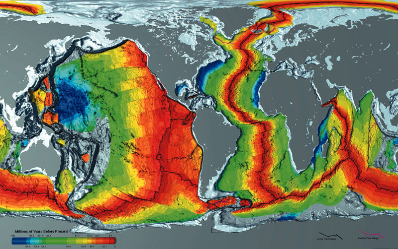 |
Figure 5: Rocks from the ocean floor indicate
youngest sea floor (shown in red) exists at spreading centers along the axis of mid-ocean ridges. (from NOAA) Click to enlarge. |
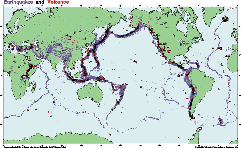
By 1968 geologists had developed a comprehensive model describing both the motions of continents and ocean floors and could confirm their ideas with many observations elevating Hess's model to the status of a scientific theory called the Theory of Plate Tectonics. A plate is a rigid slab of the lithosphere moving as a unit and may be composed of ocean floor, be entirely continental, or it may contain both oceanic and continental crust (Figure 6). Plate boundaries are defined and identified by mapping narrow belts of earthquakes, volcanoes, and young mountain ranges (Figure 7).
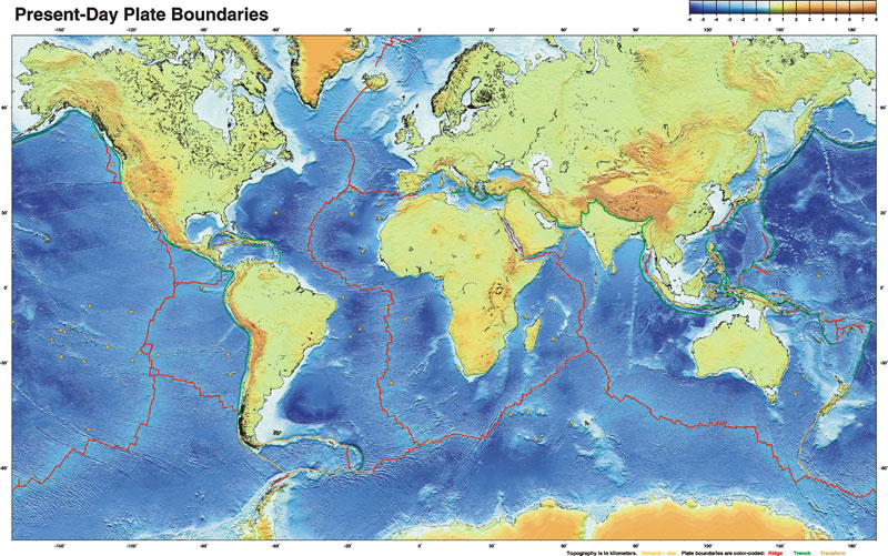
Click to enlarge
The rigid lithospheric plates on earth’s surface are constantly in motion relative to each other. The boundaries between these plates can be one of three types: divergent, convergent, or transform fault boundaries (Figure 8).
 |
Figure 8: Types of plate boundaries include divergent, convergent,
transform fault boundaries. New ocean crust is constantly being formed at divergent plate boundaries while older
ocean crust is being destroyed and recycled at convergent boundaries.
(From USGS Dynamic Earth) Click to enlarge. |
Divergent boundaries – are where plates move apart from one another (Figure 9). Most are located along the crests of oceanic ridges and can be thought of as constructive plate margins where new ocean floor is created from the upwelling of magma. As a result of this motion, oceanic ridges are formed due to the emerging less dense hot molten rock. Examples of oceanic ridges include: the Mid-Atlantic Ridge, or the East Pacific Rise.
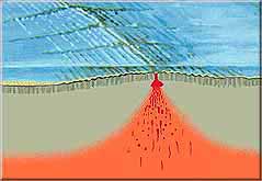 |
Figure 9: Cross section of earth
illustrating a divergent plate boundary.
(From USGS) |
Convergent boundaries – are places where plates move together or toward each other. There are three types of convergent environments depending on the kind of Earth’s crust that is involved with the convergence. The possibilities include: oceanic–oceanic convergence, oceanic-continental convergence, or continental- continental convergence. The result of this motion is either subduction of oceanic lithosphere into the asthenosphere or collision of two continental margins creating a mountain system.
- Oceanic-oceanic convergence: one plate (older, cooler, and denser) slips under the other due to subduction (Figure 10). Older portions of oceanic plates are returned to the mantle in these destructive plate margins. The subducting plate moves downward entering a high temperature and high pressure environment. This action can cause some of the descending material to melt and rise into the overriding plate. This molten material may reach the surface where it forms volcanic eruptions. The surface expression of the descending plate is an ocean trench. Oceanic-oceanic convergence can result in the formation of volcanic island arcs such as the: Aleutian, Mariana, or Tonga Islands.
Figure 10: Cross section of earth illustrating an oceanic-oceanic convergent plate boundary. (From USGS)
- Oceanic-continental convergence: Whenever continental lithosphere converges with oceanic lithosphere, the less dense continental plate will always remain above the sinking denser oceanic lithosphere (Figure 11). Examples of oceanic-continental convergence include: the U.S. Pacific Northwest where the Juan de Fuca Plate is descending under the North American Plate near Washington and Oregon creating the Cascade Mountains, or the western margin of South America creating the Peru-Chile trench and Andes Mountains.
Figure 11: Cross section of earth illustrating an oceanic-continental convergent plate boundary. (From USGS)
- Continental-continental convergence: Whenever a subducting oceanic plate also drags along with it continental lithosphere, the subduction process will continue eventually bringing in contact the overriding continental lithosphere and the continental material being dragged along with the subducting ocean floor. When this occurs neither slabs of continental lithosphere will subduct since they are both composed of buoyant granitic crust. The result is a collision between the two continental slabs (Figure 12). An example of this situation occurred when India collided with Asia and produced the Himalayas. Other older examples include formation of the Urals, Appalachians, and Alps.
Figure 12: Cross section of earth illustrating a continental -continental convergent plate boundary. (From USGS)
Transform fault boundaries – are located where one plate slides past another and no new lithosphere is created or destroyed. Most join two segments of a mid-ocean ridge as parts of prominent linear breaks in the oceanic crust known as fracture zones. A few (the San Andreas Fault and the Alpine fault of New Zealand) cut through continental crust.
 |
Figure 13: Transform fault plate boundaries. Several examples exist on ocean floors
as seen here on the Pacific Ocean floor. The San Andreas Fault is one example of a transform fault boundary
that occurs on continental lithosphere (From USGS). Click to enlarge. |
Tracking Plate Motion from Space
Today we can track the current direction and speed of plate motion with ground surveying techniques using laser-electronic instruments and by space-based methods such as with satellite networks. Since plate motions are at a global scale, they are best measured by satellite-based methods. The three most commonly used space-based techniques are: very long baseline interferometry (VLBI), satellite laser ranging (SLR), and the Global Positioning System (GPS). Among these three techniques, GPS has been the most useful for studying plate motions to date.
The GPS satellite network includes twenty-four satellites that are currently in orbit 20,000 km above the Earth as part of the NavStar system of the U.S. Department of Defense. These satellites continuously transmit radio signals back to Earth. To determine a precise position on Earth (longitude, latitude, elevation) triangulation is used. From any one position on earth one must simultaneously receive signals from at least four satellites, recording the exact time and location of each satellite when its signal was received. By repeatedly measuring distances between specific points, geologists can determine if there has been active movement between plates.
Plate motion can be measure as relative movement or absolute movement. Absolute plate movement is the motion of a plate with respect to the Earth’s deep interior (Figure 14). Relative movement refers to the movement between two plates at a given point on the plate boundary. For every pair of plates their relative motion is defined by a direction and a magnitude. This movement has a magnitude of typically tens of mm per year (Figure 15). It is relative plate movement that determines the amount and type of earthquake and volcanic activity present along a plate boundary.
Click to enlarge.

Click to enlarge.