IMAPP Remote Sensing Workshop

28 Feb. - 2 Mar. 2006

Andøya Rocket Range, Andenes, Norway

Useful Material Handout

Table: Summary of Hydra Commands

Hydra menu

Displays world map with image control functions indicated on the bottom

Reset

Zoom in (left click plus drag)

Zoom out (left click plus drag)

Rubber band zoom (left click plus drag to create box for enlargement)

Translate (left click plus drag)

Pick image (left click plus drag displays location of the chosen pixel)

Subset image (left click plus drag to create subset of image; this is automatically transferred from Hydra into the Multichannel viewer when both are engaged)

Also shows menus for Data, Settings, and Start at top

Data menu:

Local allows you to scroll through local directories to find data

· Remote allows you to find an AIRS granule from a remote server (a) MODIS Direct Broadcast or (b) Goddard DAAC

Exit

After a MODIS or AIRS granule is selected hydra displays the infrared window on a world map

Settings menu

Set color range (left click shows VisAD histogram – color range can be altered with

· a right click plus drag at either end of the color scale)

o Set color scale gives choice of color, grey, or inverse grey (which produces white clouds)

Start opens Multichannel Viewer

· wherein a spectra (wavenumber on x-axis and radiance on y-axis) is displayed along with a spectral band superimposed on a world map. Left click on pick image in bottom tool bar the allows you to see the pixel value for a given lat-lon (using left click and drag)

Tools menu

Linear Combinations opens channel combination tool display where you can specify

· linear combinations of spectral bands a,b,c and d

· (a ±´¸ b) ±´¸ (c ±´¸ d)

o Compute creates an image of the selected linear combination (indicate at the

§ bottom preference for this linear combination to be x- or y-axis in the scatter plot)

Scatter allows you to create a scatter plot of the chosen x- and y-axis linear

· combinations. Five color area boxes (or area curves) can be initiated at

o the bottom of the scatter plot; a left click drag in the scatter plot highlights the chosen points in the scatter plot and simultaneously in the x- and y-axis images. Conversely left click drag in the x- or y- axis images shows the locations of the chosen pixels in the scatter plot. Each color area box (or area curve) can be erased with a left click when the color box is engaged; after erasure another area box (or area curve) can be selected for this color.

Transect allows you to create a line on the image and see the temperatures or

· radiances of the transect. This is enabled with a left click drag.

Capture Display makes jpeg in location you specify

Statistics allows you to display min and max values and locations on image (toggle on

· or off)

Settings menu

Set color range opens VISAD histogram of brightness temperature (BT) values

Radiance – BT allows you to select radiance or brightness temperature in the display

Projection allows you to put the data in a given projection (mercator is the default)

Set Color Scale gives you the choice of color, grey, or inverted grey

Figure 1 Black: Earth IR Emission Spectrum at high spectral resolution. Red VIIRS IR bands. Green: MODIS IR bands

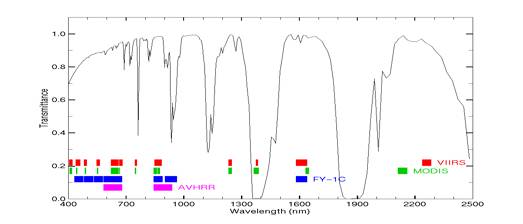
Figure 2. Black: Atmospheric Transmittance. Red: VIIRS bands. Green: MODIS bands.

Figure 3. Top left: Surface Albedo; Top middle: Surface Reflactance. Top right: MODIS Weighting functions. Bottom left: Absorpion Coefficient for Water and ICE. Bottom Middle: Surface Emissivity in the IR portion of the Spectrum. Bottom right: Absorption characteristics for water and chlorophyll.

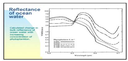
Figure 4. Reflectance of Ocean Water.

Figure 5. Planck functions for different black body temperature values.

MODIS Instrument Characteristics

MODIS Reflected Solar Bands				MODIS Thermal Emissive Bands
Band	Wavelength (micron)	Primary application	Band	Wavelength (micron)	Primary application
1,2	0.645, 0.866	Land, Clouds	20-23	3.75(2), 3.95, 4.05	Surface / cloud temperature
3,4	0.470, 0.555	Land, Clouds	24,25	4.46, 4.51	Atmospheric temperature
5-7	1.24, 1.64, 2.13	Land, Clouds	27,28	6.71, 7.32	Water vapor
8-10	0.450, 0.443, 0.490	Ocean color	29	8.55	Surface / cloud temperature
11-13	0.531, 0.565, 0.653	Ocean color	30	9.73	Ozone
14-16	0.681, 0.750, 0.865	Ocean color	31,32	11.03, 12.02	Surface / cloud temperature
17-19	0.905, 0.936, 0.940	Water vapor	33,34	13.33, 13.63	Cloud top properties
26	1.375	Cirrus clouds	35,36	13.93, 14.23	Cloud properties

Table: Summary of some MODIS Cloud Tests

Scene	Solar/Reflectance	Thermal	Comments
Low cloud over water	R0.86, R0.67/R0.86, BT11-BT3.7	Difficult, Compare BT11 to daytime mean clear-sky values of BT11; BT11 in combination with BT difference tests; Over oceans, expect a relationship between [BT11-BT8.6], [BT11-BT12] due to water vapor correlation to SST	Spatial and temporal uniformity tests sometimes used over water scenes; Beware of Sun-glint regions
High Thick cloud over water	R1.38, R0.86, R0.67/R0.86,	BT11 ; BT13.6 ; BT6.7 [BT11-BT8.6], [BT11-BT12]	Easy, good contrast in vis and IR
High Thin cloud over water	R1.38, DR0.86, [R0.65–R1.6]/[R0.65+R1.6];	BT6.7 ; BT13.9 [BT11-BT12], [BT3.7-BT12], [BT8.6-BT11]	For R1.38, be careful of surface reflectance for atmospheres with low total water vapor amounts. For BT difference tests, beware of variations in surface emissivity.
Low cloud over snow	[R0.65–R1.6]/[R0.65+R1.6]; R2.1 back up to 1.6 [BT11-BT3.7]<<0	Difficult, look for inversions in clr sky BT11-BT6.7 < 0	NDSI (Normalized Difference Snow Index) is ratio test. R2.1 is also dark over snow and bright for low cloud.
High thick cloud over snow	R1.38; [R0.65–R1.6]/[R0.65+R1.6]	BT11 ; BT13.6 ; BT6.7 Look for inversions, suggesting cloud-free.	Usually easy
High thin cloud over snow	R1.38; [R0.65–R1.6]/[R0.65+R1.6]	BT11 ; BT13.6 ; BT6.7 Look for inversions, suggesting clear sky.
Low cloud over vegetation	R0.86, R0.67/R0.87, BT11-BT3.7; [R0.86–R0.65] /[R0.86+R0.65]	Difficult, BT11 in combination with BT difference tests.	NDVI (Normalized Difference Vegetation Index). Other ratio tests also are good. Can make tests a function of ecosystem.
High Thick cloud over vegetation	R1.38, R0.86, R0.67/R0.86, [R0.86–R0.65] /[R0.86+R0.65]	BT11 ; BT13.9; BT6.7 [BT11-BT8.6], [BT11-BT12]	Can make tests a function of ecosystem to account for variations in surface emittance and reflectance.
High Thin cloud over vegetation	R1.38, R0.86, R0.67/R0.86, [R0.86–R0.65] /[R0.86+R0.65]	BT13.9; BT6.7 [BT11-BT8.6], [BT11-BT12]	Beware of variations in surface emittance and reflectance.
Low cloud over bare soil	R0.86, R0.67/R0.86, [BT11-BT3.7]	BT11 in combination with brightness temperature difference tests. [BT3.7-BT3.9]	Difficult due to brightness and spectral variation in surface emissivity. Surface reflectance at 3.7 and 3.9 mm is similar.
High Thick cloud over bare soil	R1.38, R0.86, R0.67/R0.86	BT13.9; BT6.7 BT11 in combination with brightness temperature difference tests.
High Thin cloud over bare soil	R1.38, R0.86, R0.67/R0.87, [BT11-BT3.7]	BT13.9; BT6.7 BT11 in combination with brightness temperature difference tests, for example [BT3.7-BT3.9]	Difficult; be careful of surface reflectance at 1.38 mm. and variations in surface emittance.
Cloud-top pressure		Channels in absorption band of carbon dioxide (13-14mm)	CO2 slicing
Cloud phase	Combination of R0.86; R1.6 and R2.1	[BT8.6 – BT11]>0 for ice and <0 for water. [BT11 – BT12] for water clouds > [BT8.6 – BT11]. Conversely, [BT8.6 – BT11] for ice cloud > [BT11 – BT12].	Watch out for cloud overlap Determine phase by using observations that test for high cloud versus those that test for low.
Cloud particle size	Combination of R0.86; R1.6 , R2.1; & R3.7	[BT8.6 – BT11] values versus [BT11 – BT12] is useful for thin high clouds.	Arches