Radiation Objective:
Matlab Objective:
- Work with visible, near-infrared, and infrared images from MAS.
- Determine MAS channels for detecting clouds.
- Display image combinations as scatter plots.
The MODIS Airborne Simulator (MAS) is an airborne scanning spectrometer that acquires high spatial resolution imagery of cloud and surface features from its vantage point on-board a NASA ER-2 high-altitude research aircraft. You can learn more about this instrument at http://ltpwww.gsfc.nasa.gov/MODIS/MAS/Home.html
- Perform simple image processing on MAS data (addition, subtraction, division).
- Use the 'image', 'caxis', and 'colorbar' commands to plot MAS data.
- Make scatter plots.
Part I. Displaying MAS data
A) Download the following MAT file to your local directory: lab9.mat (to get this file, try holding down the shift key and clicking the mouse button). This can be loaded into Matlab using the 'load' command. lab9.mat contains 6 variables related to MAS data for a scene near Denver, Colorado. (When Pete downloads this file you will not have to download the data, but you will have to change the load command to point to the correct directory.)
wv - Wavelength (in mm) of the 5 MAS bands
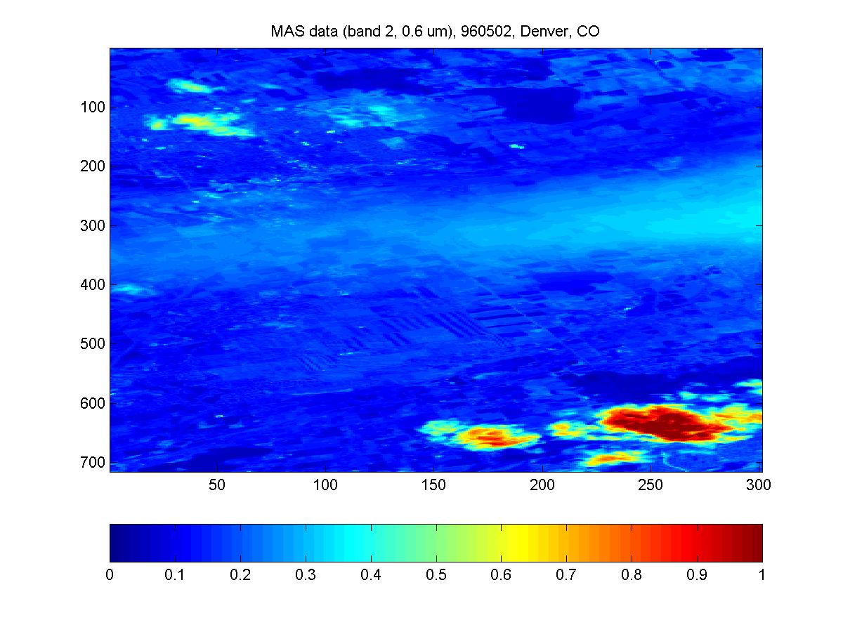
ref0_6 - Reflectance at 0.6 mm.
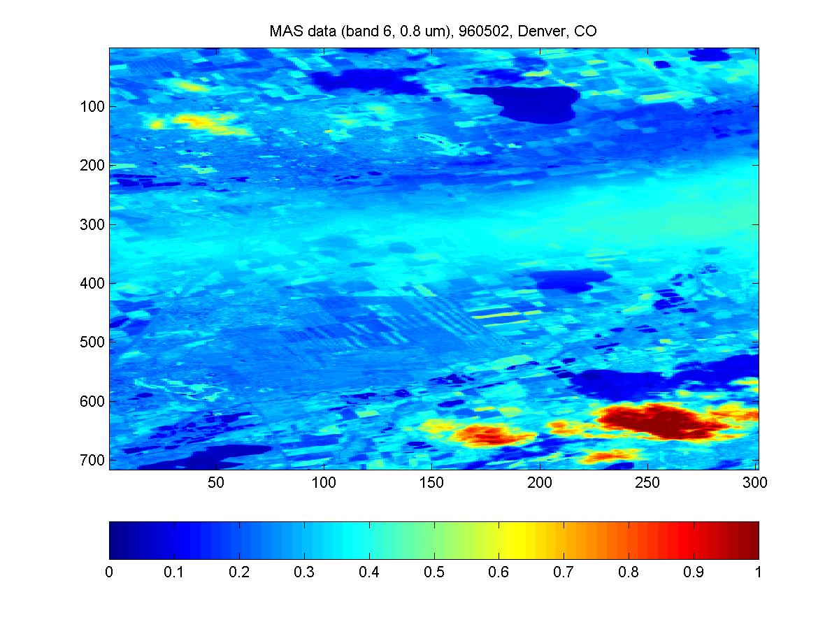
ref0_8 - Reflectance at 0.8 mm.
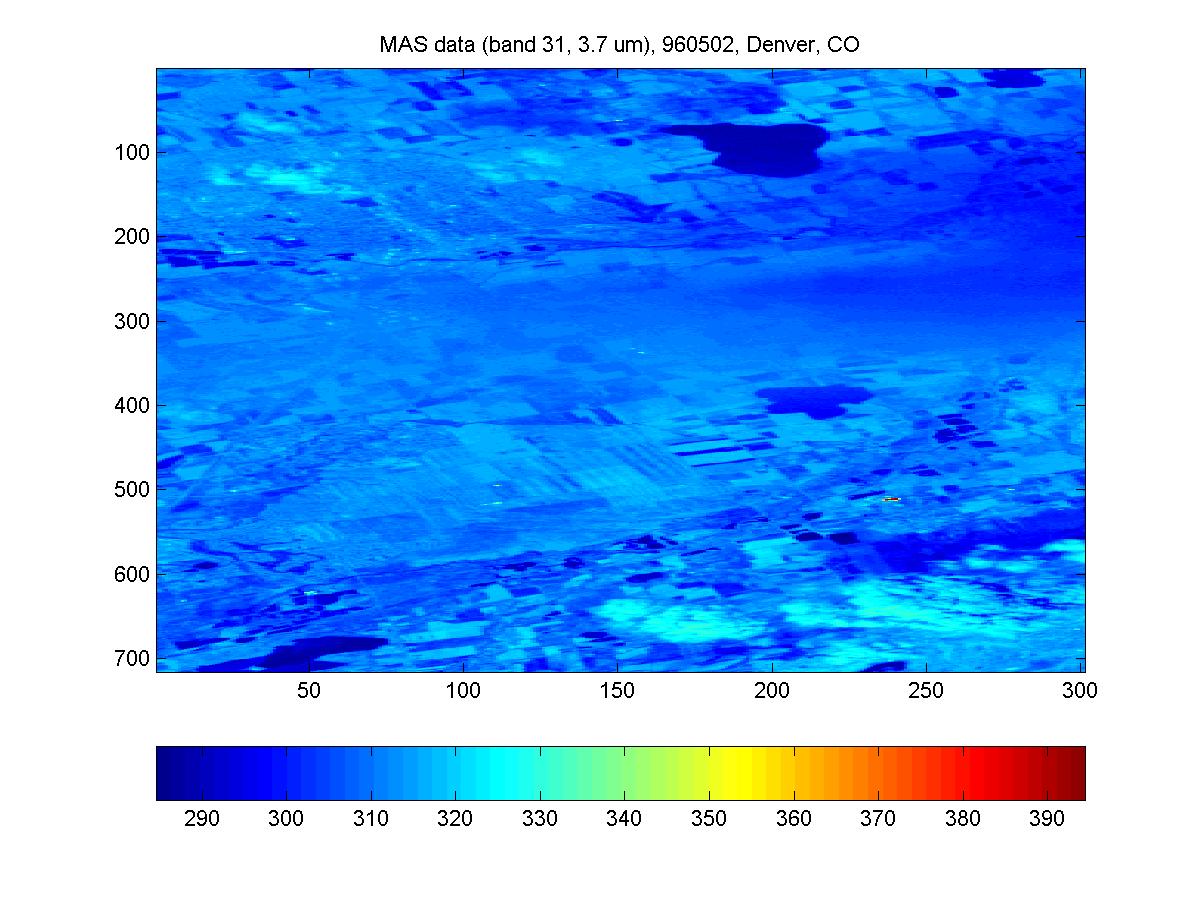
bt3_7 - Brightness temperature at 3.7 mm.
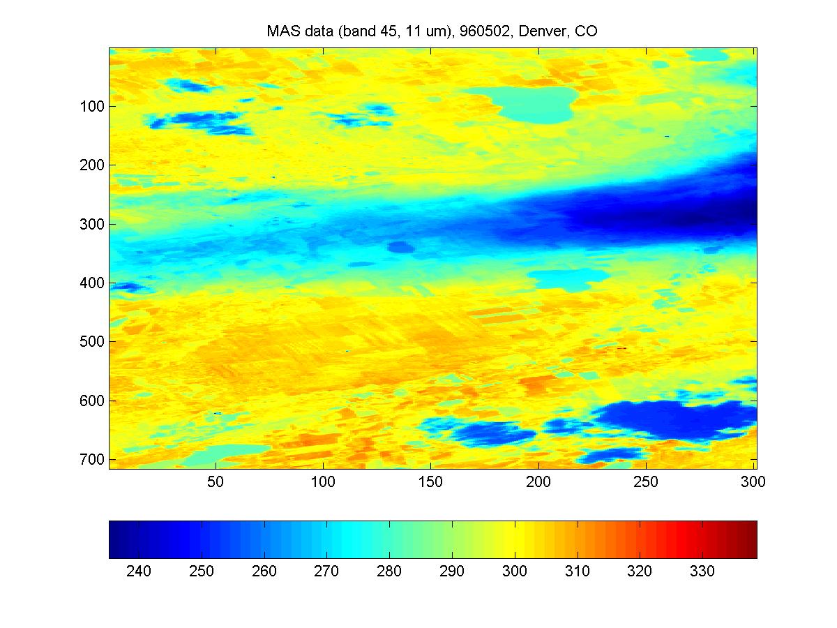
bt11 - Brightness temperature at 11 mm.
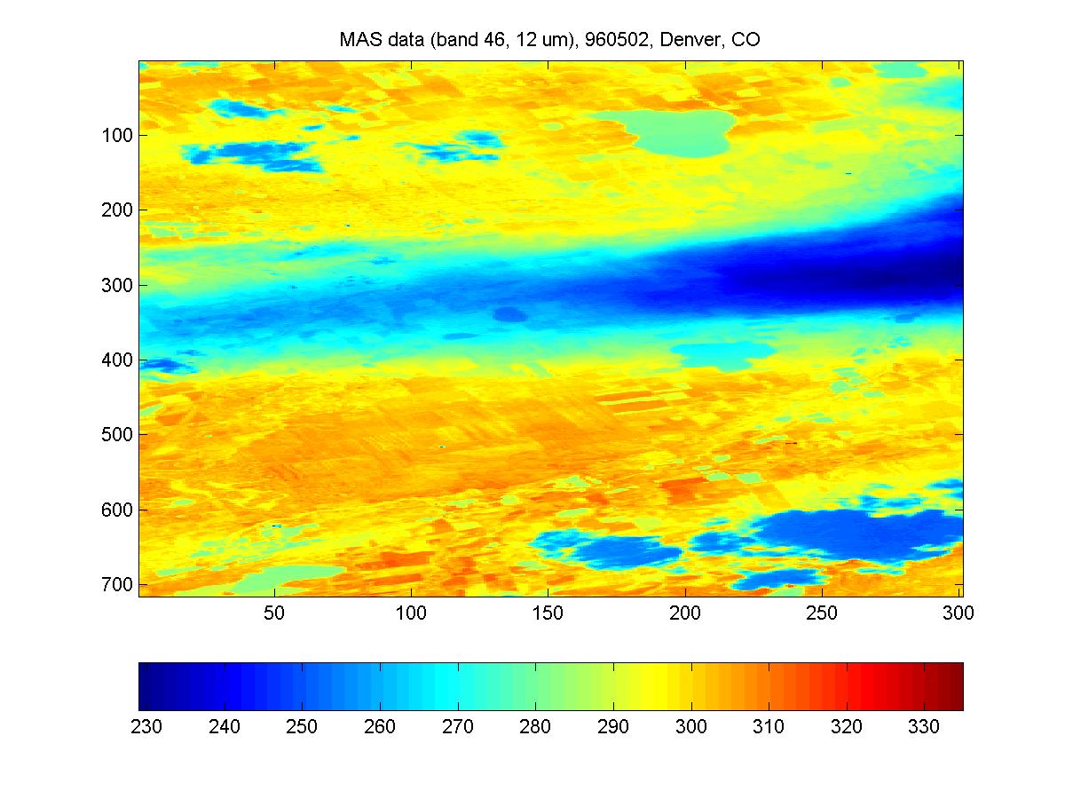
bt12 - Brightness temperature at 12 mm.ref0_6, ref0_8, bt3_7, bt11, and bt12 are arrays of dimension, 716 x 301; there are 716 times (or scans) and 301 pixels per scan.
Plot these images using the MATLAB script masread_cloud. This script produces 7 figures (1 | 2 | 3| 4 | 5 | 6 | 7| )The program utilizes the following commands: (Remember to turn in your additions to this script!) Note the caxis command is not needed for bt3_7, bt11, and bt12. (On Unix machines, you may have to place the mouse cursor inside the figure window to get the colors to look right.)
h = image(ref0_6);
set(h,'CDataMapping','scaled');
caxis([0 1])
colorbar('horiz')
title('MAS data (band 2, 0.6 um), 960502, Denver, CO')Describe these images by stating for each band where you see the surface and where you see clouds. What values of reflectance are typical for land? For clouds? What are typical values of brightness temperatures for the land and clouds? Are the clouds in these images made of water droplets or ice crystals? Justify your answer. [HINT: Use the colorbar on your 11-mm figure.]
Part II. Cloud Detection by Threshold
Choose three of these channels to determine a "mask" for clouds; a mask tells you where clouds are in the image. Explain your choices. What reflectance or brightness temperature thresholds would you use for cloud detection for this scene in each of your channels?
Part III. Cloud Detection using Combinations of Channels
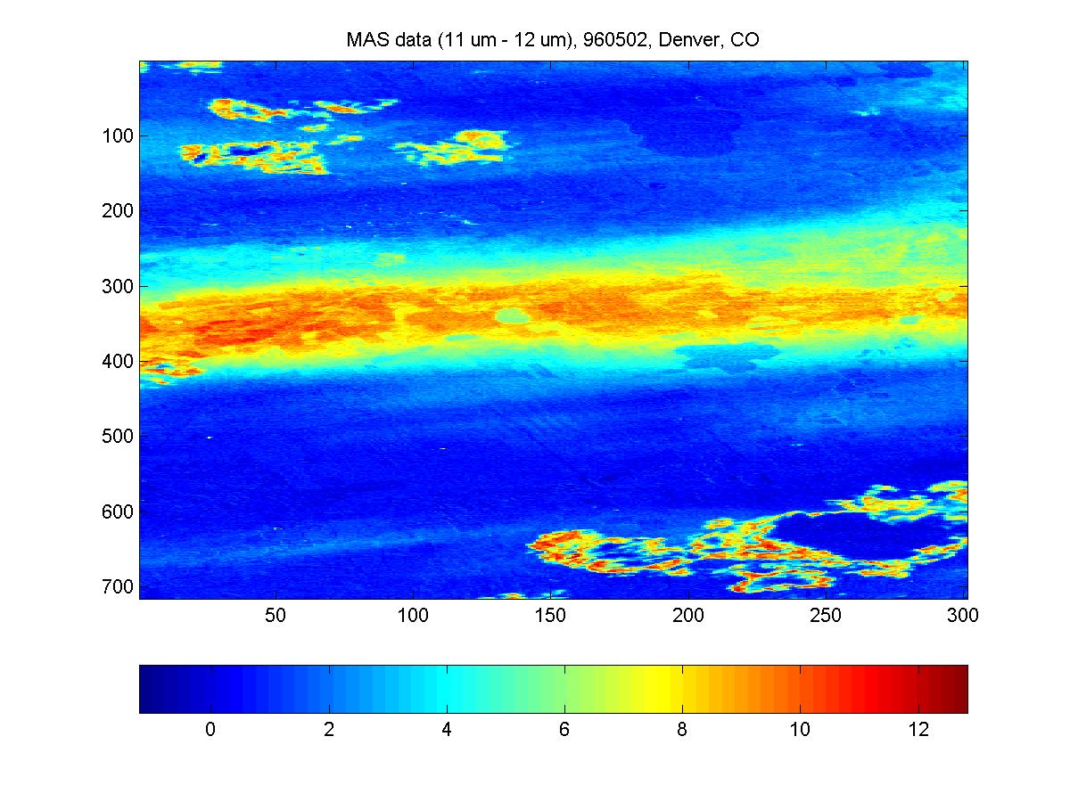
Combinations of spectral channels can be used to retrieve cloud properties. Plot these band combinations, and choose two out the three that would provide the most complete cloud detection. Justify your choices of bands.
ref0_8 / ref0_6
bt3_7 - bt11
bt11 - bt12What cloud thresholds would you use in your selected band combinations? Justify your threshold values.
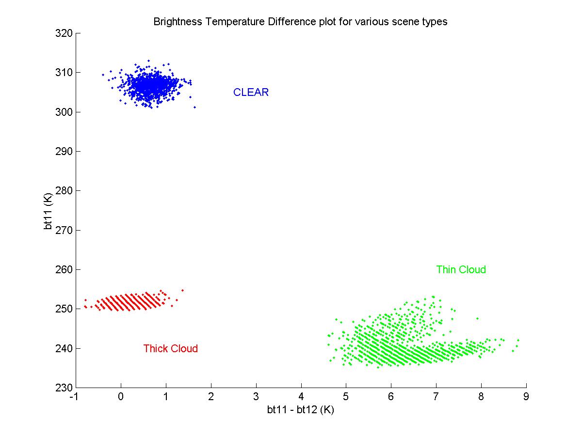
Part IV. Cloud Detection using Scatter Plots
Select portions of the image that pertain to a particular type of scene (e.g. clear, thin cloud, thick cloud, low cloud, high cloud). Plot these as a scatter plot (on the same graph) with an x-axis of (bt11 - bt12) and a y-axis of (bt11). Notice that the origin of the image is in the upper left corner of the plot rather than the typical location in the lower left corner. Due to the way that Matlab plots images, the rows of the 716x301 arrays are actually columns in the images that you've created above. Be careful to swap rows and columns in the plot command as I have below. As an example, to create a plot of a section of the lower left corner and the upper right corner, try
figure
hold on
plot(bt11(700:716,1:25)-bt12(700:716,1:25),bt11(700:716,1:25),'b.') % lower left
plot(bt11(1:25,275:301)-bt12(1:25,275:301),bt11(1:25,275:301),'r.') % upper right
hold offNote that I've used different colors for different portions of the image. This may be useful to designate different types of scenes.
On the graph, label the different scene types. Why do they occur where they do?
Part V. Summary
Discuss the advantages and disadvantages of the three cloud detection techniques used in parts II, III, and IV.